library(tidyverse) # Load the tidyverse

german_polls <- read_csv("data/german_polls.csv")
view(german_polls)8 Reshaping data
The analysis of your data is usually not the part of your project that takes longer : it is data wrangling. Your data have to be cleaned in order to be analyzed. This mean that you have a tidy datasets. Here we focus how we can combine and reshape different datasets in order to use them properly. I will use polling data of different political parties.
8.1 Reshaping with pivot_longer() and pivot_wider()
Datasets can be in long (many rows, few columns) or wide formats (few rows, many columns). Depending of what our unit of analysis is, we can reshape our datasets in different formats. In german_polls, the vote intentions of each party are stored in different columns. But we could also have a column with parties and a column with voting intention.
(german_long <- german_polls |>
  pivot_longer(
    # Select which columns to pivot
    cols = c(Union, FDP, LINKE, SPD, PIRATEN, AfD, GRUENE),
    # Choose a name for the new column with all of the parties
    names_to = "party",
    # Choose a name for the new column with the vote intentions
    values_to = "intention"
  ))
# A tibble: 24,115 × 6
date firm date_from sample_size party intention
<date> <chr> <date> <dbl> <chr> <dbl>
1 2005-09-22 FG Wahlen 2005-09-20 1345 Union 37
2 2005-09-22 FG Wahlen 2005-09-20 1345 FDP 8
3 2005-09-22 FG Wahlen 2005-09-20 1345 LINKE 8
4 2005-09-22 FG Wahlen 2005-09-20 1345 SPD 35
5 2005-09-22 FG Wahlen 2005-09-20 1345 PIRATEN NA
6 2005-09-22 FG Wahlen 2005-09-20 1345 AfD NA
7 2005-09-22 FG Wahlen 2005-09-20 1345 GRUENE 8
8 2005-10-06 FG Wahlen 2005-10-04 1259 Union 39
9 2005-10-06 FG Wahlen 2005-10-04 1259 FDP 7
10 2005-10-06 FG Wahlen 2005-10-04 1259 LINKE 9
# ℹ 24,105 more rowsgerman_long# A tibble: 24,115 × 6
date firm date_from sample_size party intention
<date> <chr> <date> <dbl> <chr> <dbl>
1 2005-09-22 FG Wahlen 2005-09-20 1345 Union 37
2 2005-09-22 FG Wahlen 2005-09-20 1345 FDP 8
3 2005-09-22 FG Wahlen 2005-09-20 1345 LINKE 8
4 2005-09-22 FG Wahlen 2005-09-20 1345 SPD 35
5 2005-09-22 FG Wahlen 2005-09-20 1345 PIRATEN NA
6 2005-09-22 FG Wahlen 2005-09-20 1345 AfD NA
7 2005-09-22 FG Wahlen 2005-09-20 1345 GRUENE 8
8 2005-10-06 FG Wahlen 2005-10-04 1259 Union 39
9 2005-10-06 FG Wahlen 2005-10-04 1259 FDP 7
10 2005-10-06 FG Wahlen 2005-10-04 1259 LINKE 9
# ℹ 24,105 more rowsgerman_intentions <- german_long |>
group_by(date, party) |>
summarise(intention = mean(intention, na.rm = T))`summarise()` has grouped output by 'date'. You can override using the
`.groups` argument.We can also reshape the dataset to put it back on wide format.
(german_wide <- german_long |>
  pivot_wider(
    names_from = party,
    values_from = intention
  ) |>
  unnest())
# A tibble: 3,445 × 11
date firm date_from sample_size Union FDP LINKE SPD PIRATEN AfD
<date> <chr> <date> <dbl> <dbl> <dbl> <dbl> <dbl> <dbl> <dbl>
1 2005-09-22 FG W… 2005-09-20 1345 37 8 8 35 NA NA
2 2005-10-06 FG W… 2005-10-04 1259 39 7 9 34 NA NA
3 2005-10-13 FG W… 2005-10-11 1280 38 8 8 35 NA NA
4 2005-10-27 FG W… 2005-10-25 1269 37 9 8 35 NA NA
5 2005-11-10 FG W… 2005-11-08 1230 36 9 9 33 NA NA
6 2005-11-24 FG W… 2005-11-22 1298 37 9 8 34 NA NA
7 2005-12-08 FG W… 2005-12-06 1237 38 9 8 34 NA NA
8 2006-01-12 FG W… 2006-01-10 1249 39 9 8 33 NA NA
9 2006-01-26 FG W… 2006-01-24 1279 41 8 8 33 NA NA
10 2006-02-16 FG W… 2006-02-14 1260 41 8 7 32 NA NA
# ℹ 3,435 more rows
# ℹ 1 more variable: GRUENE <dbl># How many times the Greens have been higher in the polls than SPD ?
german_wide |>
mutate(left = GRUENE > SPD) |>
count(left)# A tibble: 2 × 2
left n
<lgl> <int>
1 FALSE 2692
2 TRUE 7539 Combining with bind_rows
Now I want to combine this data from Germany with the same data from the spanish case.
spain_polls <- read_csv("data/spain_polls.csv")Rows: 1414 Columns: 22
── Column specification ────────────────────────────────────────────────────────
Delimiter: ","
chr (1): firm
dbl (19): PP, PSOE, ERC, PNVEAJ, CC, BNG, Cs, VOX, Podemos, EHBildu, PACMA,...
date (2): date, date_from
ℹ Use `spec()` to retrieve the full column specification for this data.
ℹ Specify the column types or set `show_col_types = FALSE` to quiet this message.(spain_polls <- spain_polls |>
pivot_longer(
# Select which columns NOT to pivot
cols = -c(date, firm, date_from, sample_size),
# Choose a name for the new column with all of the parties
names_to = "party",
# Choose a name for the new column with the vote intentions
values_to = "intention"
))# A tibble: 25,452 × 6
date firm date_from sample_size party intention
<date> <chr> <date> <dbl> <chr> <dbl>
1 2011-12-15 Metroscopia 2011-12-14 1000 PP 44.9
2 2011-12-15 Metroscopia 2011-12-14 1000 PSOE 28.4
3 2011-12-15 Metroscopia 2011-12-14 1000 ERC NA
4 2011-12-15 Metroscopia 2011-12-14 1000 PNVEAJ NA
5 2011-12-15 Metroscopia 2011-12-14 1000 CC NA
6 2011-12-15 Metroscopia 2011-12-14 1000 BNG NA
7 2011-12-15 Metroscopia 2011-12-14 1000 Cs NA
8 2011-12-15 Metroscopia 2011-12-14 1000 VOX NA
9 2011-12-15 Metroscopia 2011-12-14 1000 Podemos NA
10 2011-12-15 Metroscopia 2011-12-14 1000 EHBildu NA
# ℹ 25,442 more rowsI also add a country variable to add information on the country of the two datasets.
spain_long <- spain_polls |> mutate(country = "Spain")
german_long <- german_long |> mutate(country = "Germany")

view(spain_long)
view(german_long)
And combine the two with bind_rows()
polls <- bind_rows(spain_long, german_long)polls |>
filter(party %in% c("AfD", "PP", "Union", "VOX")) |>
ggplot(aes(date, intention, color = party, group = party)) +
geom_smooth(se = F) +
facet_wrap(~ country)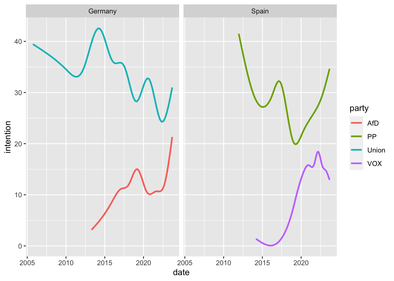
10 Going further
polls |>
  # Compute the mean of voting intention for each party/date
  summarise(intention = mean(intention, na.rm = T), .by = c(country, date, party)) |>
  # Compute party ranking for each date
  mutate(rank = row_number(-intention), .by = date) |>
  # Keep only the party that leads the polls
  filter(rank == 1) |>
  # Count how manu times each party arrived first
  count(rank, party, sort = T)
# A tibble: 7 × 3
rank party n
<int> <chr> <int>
1 1 Union 2373
2 1 PP 444
3 1 PSOE 174
4 1 SPD 79
5 1 GRUENE 10
6 1 Cs 6
7 1 Podemos 5