# Load packages

needs(tidyverse, janitor, haven, broom, labelled, scales, infer)

# Load the data

fes <- read_dta("data/fes2022v4bis.dta")

annual <- read_dta("data/elipss_annual.dta")12 Testing relationships
In social sciences, our primary interest lies in understanding how certain variables vary across different groups. This session primarily focuses on bivariate relationships. When analyzing data, our objective is often to measure the association between two variables. For example, are men more likely to vote for radical right parties than women? Do autocratic regimes engage in warfare more frequently than democracies? Do individuals with more information tend to hold stronger beliefs in the reality of climate change compared to others? In this context, we are solely concentrating on relationships and not causality. Investigating causality would entail understanding the exact nature of the relationship and accounting for other variables that may influence this association.
Precisely, when examining these relationships, our main concern is inference. Typically, our analysis is based on a sample taken from the population under study, which means that our results are contingent on this specific sample. However, our ultimate goal is to make general statements or draw conclusions about the larger population. To determine if the observed association in our data can be generalized, we need to conduct statistical tests. These tests provide us with the best estimate of the “true” value of the population parameter and assess the level of confidence we have in our findings. They indicate how different the observed association in our data might be from the actual population relationship. By performing these statistical tests, we can make more reliable inferences about the broader population based on the sample we have analyzed.
Our primary objective here is inference. We aim to determine whether the relationship we observe in the data is real or merely a result of random chance. To do this, we formulate a null hypothesis: that the relationship we observe is due to random chance. Typically, we seek to reject this null hypothesis and provide evidence for our alternative hypothesis that this effect is not random. To achieve this, we conduct a test that yields a p-value, which represents the probability that our observed data would occur if the null hypothesis were true.
To explore how to do this in R, we will use data from the 2022 french electoral study. This dataset was collected following the last french presidential election and contains variable on voting behavior. Before testing the relationship between different variables, I will also cover various data wrangling steps that are often necessary before analysing the data,such as joining dataframes, recoding variables and managing missing values.
12.1 Joining datasets
In many instances, we encounter data originating from different datasets that share common variables. In this context, I have two datasets concerning French voters. The first dataset is an annual survey that comprises information regarding the socio-demographic characteristics of the respondents. The second dataset is a panel survey conducted during the most recent presidential election, providing data about the voting choices of the respondents. Both datasets pertain to the same individuals and include a unique identifier (UID) that enables us to correlate the two datasets. Our objective is to amalgamate these two datasets into a single one that encompasses both the socio-demographic characteristics and the voting choices of the respondents. To accomplish this, we must merge the two datasets. Note that this is different from binding datasets together as we already did before with bind_rows() where we binded datasets having the same columns but not the same observations.
Let’s start by loading a bunch of packages we will use today and the two datasets I just described.
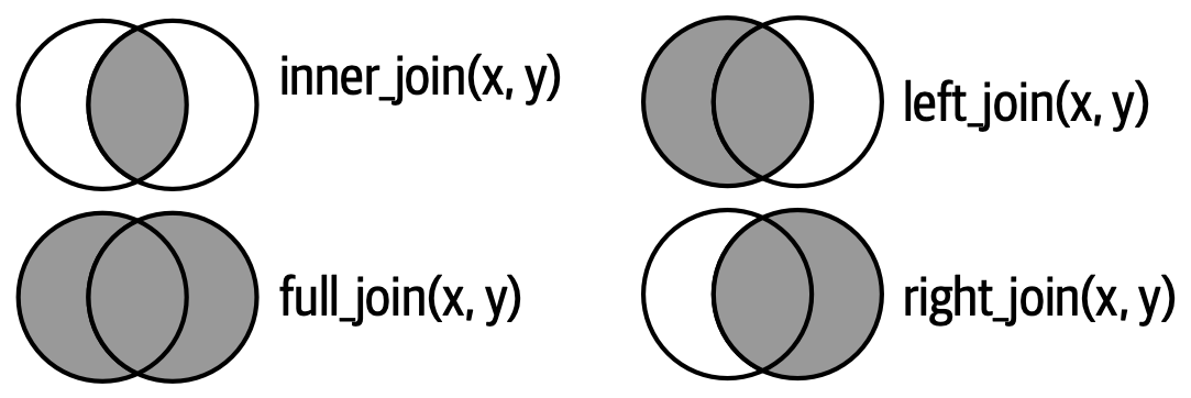
To join them together, we will use the left_join() function from the dplyr package. This function is used to combine two datasets by matching the values of one or more variables in each dataset. The first dataset is the one that we want to keep all the observations from. The second dataset is the one that we want to add observations from. In our case, we want to keep all the observations from the fes dataset and add the variables from the annual dataset. The by argument specifies the variable(s) that will be used to match observations in the two datasets. In our case, we will use the UID variable that is common to both datasets.
fes2022 <- left_join(fes, annual, by = c("UID")) # Join the two datasets by the UID variableThe left_join() function is indeed one of the most commonly used methods for joining data in R. However, it’s important to note that there are several other types of joins that can be applied, each with its own specific use case. If you’d like to delve deeper into how these joins work, I recommend checking out theR for data science book’s explanation of these concepts. These diagrams below shows the different types of joins that can be performed with the dplyr package.
If we check the names of our columns, we can now see that we have in our new dataset, the columns of both previous datasets with the same number of observations.
colnames(fes2022) [1] "UID" "fes4_Q01" "fes4_Q02a"
[4] "fes4_Q02b" "fes4_Q02c" "fes4_Q02d"
[7] "fes4_Q02e" "fes4_Q02f" "fes4_Q02g"
[10] "fes4_Q03" "fes4_Q04a" "fes4_Q04b"
[13] "fes4_Q04c" "fes4_Q04d" "fes4_Q04_DO_Q04a"
[16] "fes4_Q04_DO_Q04b" "fes4_Q04_DO_Q04c" "fes4_Q04_DO_Q04d"
[19] "fes4_Q05a" "fes4_Q05b" "fes4_Q05c"
[22] "fes4_Q05_DO_Q05a" "fes4_Q05_DO_Q05b" "fes4_Q05_DO_Q05c"
[25] "fes4_Q06" "fes4_Q07a" "fes4_Q07b"
[28] "fes4_Q07d" "fes4_Q07e" "fes4_Q07f"
[31] "fes4_Q07g" "fes4_Q07_DO_Q07a" "fes4_Q07_DO_Q07b"
[34] "fes4_Q07_DO_Q07c" "fes4_Q07_DO_Q07d" "fes4_Q07_DO_Q07e"
[37] "fes4_Q07_DO_Q07f" "fes4_Q07_DO_Q07g" "fes4_Q08a"
[40] "fes4_Q08b" "fes4_Q09" "fes4_Q10p1_a"
[43] "fes4_Q10p1_b" "fes4_Q10p2_a" "fes4_Q10p2_b"
[46] "fes4_Q10lh1_a" "fes4_Q10lh1_c" "fes4_Q11a"
[49] "fes4_Q11b" "fes4_Q11c" "fes4_Q12"
[52] "fes4_Q13" "fes4_Q14a" "fes4_Q14b"
[55] "fes4_Q14c" "fes4_Q14d" "fes4_Q15"
[58] "fes4_Q16a" "fes4_Q16b" "fes4_Q16c"
[61] "fes4_Q16d" "fes4_Q16e" "fes4_Q16f"
[64] "fes4_Q16g" "fes4_Q16h" "fes4_Q17a"
[67] "fes4_Q17b" "fes4_Q17c" "fes4_Q17d"
[70] "fes4_Q17e" "fes4_Q17f" "fes4_Q18a"
[73] "fes4_Q18b" "fes4_Q18c" "fes4_Q18d"
[76] "fes4_Q18e" "fes4_Q18f" "fes4_Q18g"
[79] "fes4_Q18h" "fes4_Q19" "fes4_Q22"
[82] "fes4_Q23a" "fes4_Q23b" "fes4_Q23c"
[85] "fes4_Q23d" "fes4_Q24" "fes4_Q25a"
[88] "fes4_Q25b" "fes4_Q26a" "fes4_Q26b"
[91] "fes4_Q27a" "fes4_Q27b" "fes4_Q27c"
[94] "fes4_Q27d" "fes4_bloc_q25_DO_Q25a" "fes4_bloc_q25_DO_Q25b"
[97] "fes4_bloc_q26_DO_Q26a" "fes4_bloc_q26_DO_Q26b" "cal_AGE"
[100] "cal_DIPL" "cal_SEXE" "cal_TUU"
[103] "cal_ZEAT" "cal_AGE1" "cal_AGE2"
[106] "cal_NAT" "cal_DIPL2" "panel"
[109] "VAGUE" "POIDS_fes4" "PDSPLT1_fes4"
[112] "PDSPLT2_fes4" "POIDS_INIT" "PDSPLT_INIT1"
[115] "PDSPLT_INIT2" "eayy_a1" "eayy_a2a_rec"
[118] "eayy_a2a_rec2" "eayy_a3_rec" "eayy_a3b_rec"
[121] "eayy_a3c_rec" "eayy_a3d" "eayy_a3e_rec"
[124] "eayy_a4" "eayy_a5" "eayy_a5c_rec"
[127] "eayy_b1" "eayy_b1_rev" "eayy_b1_sc"
[130] "eayy_b1_sccjt" "eayy_b10a" "eayy_b10aa"
[133] "eayy_b10acjt" "eayy_b11" "eayy_b11cjt"
[136] "eayy_b18_rec" "eayy_b18c" "eayy_b18ccjt"
[139] "eayy_b18cjt_rec" "eayy_b1a" "eayy_b1acjt"
[142] "eayy_b1b" "eayy_b1bcjt" "eayy_b1cjt"
[145] "eayy_b1cjt_rev" "eayy_b2_11a_rec" "eayy_b2_11acjt_rec"
[148] "eayy_b2_rec" "eayy_b25" "eayy_b25_rec"
[151] "eayy_b25cjt_rec" "eayy_b2cjt_rec" "eayy_b4_rec"
[154] "eayy_b4cjt_rec" "eayy_b5" "eayy_b5_rec"
[157] "eayy_b5a" "eayy_b5a_rec" "eayy_b5acjt"
[160] "eayy_b5c" "eayy_b5c_rec" "eayy_b5ccjt"
[163] "eayy_b5d_rec" "eayy_b6a_12a_rec" "eayy_b6a_rec"
[166] "eayy_b6b_12b_rec" "eayy_b6b_rec" "eayy_b7b_rec"
[169] "eayy_b8_rec" "eayy_b8cjt_rec" "eayy_c1_rec"
[172] "eayy_c1jeu" "eayy_c8" "eayy_c8a_rec"
[175] "eayy_c8b_rec" "eayy_d1" "eayy_d1_rec"
[178] "eayy_d2" "eayy_d2_rev" "eayy_d3"
[181] "eayy_d4_rec" "eayy_d5_rec" "eayy_d6"
[184] "eayy_d7_1" "eayy_d7_10" "eayy_d7_2"
[187] "eayy_d7_3" "eayy_d7_4" "eayy_d7_5"
[190] "eayy_d7_6" "eayy_d7_7" "eayy_d7_8"
[193] "eayy_d7_9" "eayy_d7_rev_1" "eayy_d7_rev_10"
[196] "eayy_d7_rev_11" "eayy_d7_rev_2" "eayy_d7_rev_3"
[199] "eayy_d7_rev_4" "eayy_d7_rev_5" "eayy_d7_rev_6"
[202] "eayy_d7_rev_7" "eayy_d7_rev_8" "eayy_d7_rev_9"
[205] "eayy_e1a_rec" "eayy_e1b_rec" "eayy_e1c_rec"
[208] "eayy_e1d_rec" "eayy_e1e_rec" "eayy_e1f"
[211] "eayy_e1f1_rec" "eayy_e1f2_rec" "eayy_e1g_rec"
[214] "eayy_e1h_rec" "eayy_e1i_rec" "eayy_e1j_rec"
[217] "eayy_e2a_rec" "eayy_e2auc" "eayy_e2auc_source"
[220] "eayy_e3a" "eayy_e3b" "eayy_e3c"
[223] "eayy_e3d" "eayy_e3e" "eayy_e4"
[226] "eayy_e5" "eayy_e6" "eayy_f1_rec"
[229] "eayy_f1_rev" "eayy_f1a1" "eayy_f3"
[232] "eayy_f3_rev" "eayy_f4" "eayy_f6_rec"
[235] "eayy_f6a" "eayy_f7" "eayy_f7_1"
[238] "eayy_f7_10" "eayy_f7_11" "eayy_f7_12"
[241] "eayy_f7_13" "eayy_f7_14" "eayy_f7_15"
[244] "eayy_f7_2" "eayy_f7_3" "eayy_f7_4"
[247] "eayy_f7_5" "eayy_f7_6" "eayy_f7_8"
[250] "eayy_f7_9" "eayy_f7bis_1" "eayy_f7bis_10"
[253] "eayy_f7bis_11" "eayy_f7bis_12" "eayy_f7bis_13"
[256] "eayy_f7bis_14" "eayy_f7bis_2" "eayy_f7bis_3"
[259] "eayy_f7bis_4" "eayy_f7bis_5" "eayy_f7bis_6"
[262] "eayy_f7bis_7" "eayy_f7bis_8" "eayy_f7bis_9"
[265] "eayy_f8" "eayy_f9" "eayy_g1"
[268] "eayy_g1_1" "eayy_g1_2" "eayy_g10"
[271] "eayy_g2" "eayy_g3a" "eayy_g3b"
[274] "eayy_g3c" "eayy_g3d" "eayy_g4"
[277] "eayy_g5" "eayy_g6_1" "eayy_g6_2"
[280] "eayy_g6_3" "eayy_g6_4" "eayy_h_c11"
[283] "eayy_h_teo1" "eayy_h1a" "eayy_h4"
[286] "eayy_i1" "eayy_i13a" "eayy_i13b"
[289] "eayy_i2" "eayy_i8" "eayy_j1"
[292] "eayy_k3" "eayy_pcs18" "eayy_pcs6"
[295] "eayy_pcs6cjt" "eayy_typmen5" 12.2 Renaming variables
Our examination of the column names also reveals that the variable names are not particularly informative. It can be challenging to discern the specific information represented by each variable. Since our data is in Stata format, we have the advantage of having more informative labels for these variables. These labels can be accessed by using the var_label() function provided by the labelled package. To see a bit clearer, I just create a corresponding tibble with the variable names and the labels. This code is a bit more advanced, so don’t worry if you don’t understand it all. If you want to do something similar, you can copy and paste it and just change the name of the dataset.
variables <- tibble(
  variable = names(fes2022),
  # Get the variable names
  label = var_label(fes2022) |> unlist(),
  # Get the variable labels
  categories = map(variable, ~ val_labels(fes2022[[.x]])) |> as.character() |> str_remove_all("c\\(|\\)") # Get the labels for each category
)
view(variables)
With this new tibble of variables, I can now conveniently access the information stored in my dataset. It functions much like a codebook, but I can access it directly from within RStudio. This makes it easier to understand and work with the data.
head(variables)# A tibble: 6 × 3
variable label categories
<chr> <chr> <chr>
1 UID Identifiant NULL
2 fes4_Q01 Intérêt pour la politique Beaucoup …
3 fes4_Q02a Suivi de la campagne présidentielle 2022 - Chaîne de tél… `0 jour` …
4 fes4_Q02b Suivi de la campagne présidentielle 2022- Chaîne de télé… `0 jour` …
5 fes4_Q02c Suivi de la campagne présidentielle 2022 - Radio `0 jour` …
6 fes4_Q02d Suivi de la campagne présidentielle 2022 - Lecture de jo… `0 jour` …Today, I am interested in the relationship between education levels and voting behavior in the second round of the election. So I rename these two variables with more informative names. I also rename another variable that I will use on sympathy for Emmanuel Macron.
fes2022 <- fes2022 |>
  rename(education = cal_DIPL,
         vote_t2 = fes4_Q10p2_b,
         symp_macron = fes4_Q17a)

fes2022 |> count(vote_t2)
# A tibble: 5 × 2
vote_t2 n
<dbl+lbl> <int>
1 1 [Marine Le Pen, Rassemblement national (RN)] 270
2 2 [Emmanuel Macron, La République en marche (LREM)] 808
3 3 [Vous avez voté blanc] 164
4 4 [Vous avez voté nul] 39
5 NA(a) 29412.3 Recoding variables
In addition to renaming variables, we may also need to recode variables. Let’s look at these two variables.
fes2022 |>
  count(education)
# A tibble: 4 × 2
education n
<dbl+lbl> <int>
1 1 [Diplôme supérieur] 829
2 2 [BAC et BAC+2] 286
3 3 [CAP + BEPC] 352
4 4 [Sans diplôme et non déclaré] 108Regarding our education variable, we can notice a few things :
- Our variable’s values are numbers and we might have their labels instead
- Our variable’s type is
dbl, we might want to change this to factor. - Our variable’s categories appear from the more educated to the less educative and you might want to change this order.
fes2022 <- fes2022 |>
  mutate(education = education |>
          unlabelled() |>
           forcats::as_factor() |>
           fct_relevel(
             "Sans diplôme et non déclaré", "CAP + BEPC", "BAC et BAC+2", "Diplôme supérieur"))

fes2022 |>
  count(education)
# A tibble: 4 × 2
education n
<fct> <int>
1 Sans diplôme et non déclaré 108
2 CAP + BEPC 352
3 BAC et BAC+2 286
4 Diplôme supérieur 829Now let’s look at our vote variable.
fes2022 |>
  count(vote_t2)
# A tibble: 5 × 2
vote_t2 n
<dbl+lbl> <int>
1 1 [Marine Le Pen, Rassemblement national (RN)] 270
2 2 [Emmanuel Macron, La République en marche (LREM)] 808
3 3 [Vous avez voté blanc] 164
4 4 [Vous avez voté nul] 39
5 NA(a) 294Regarding this variable, we can see that :
- We have a lot of missing values (people that have not voted)
- We have information not only of voters but alo on people who casted a blank vote or a null vote.
- We might want to rename the categories to make them more informative.
Here, I’m using the case_when() function to conditionally create a new variable. I’m reassigning the values of 1 and 2 to candidates’ names and designating all other values as NAs. I also convert the variable to factor which will make it easier to work with later on.
# Recode vote_t2
fes2022 <- fes2022 |>
  mutate(candidate_t2 = case_when( # Create a new variable called candidate_t2
    vote_t2 == 1 ~ "Le Pen", # When vote_t2 is 1, assign the value "Le Pen"
    vote_t2 == 2 ~ "Macron", # When vote_t2 is 2, assign the value "Macron"
    .default = NA_character_ # Otherwise, assign NA
  )) # Convert to factor

fes2022 |>
  count(vote_t2)
# A tibble: 5 × 2
vote_t2 n
<dbl+lbl> <int>
1 1 [Marine Le Pen, Rassemblement national (RN)] 270
2 2 [Emmanuel Macron, La République en marche (LREM)] 808
3 3 [Vous avez voté blanc] 164
4 4 [Vous avez voté nul] 39
5 NA(a) 294fes2022 |>
count(candidate_t2)# A tibble: 3 × 2
candidate_t2 n
<chr> <int>
1 Le Pen 270
2 Macron 808
3 <NA> 49712.4 Dealing with Nas
In the last code chunk, it became evident that our “vote” variable contains a considerable number of missing values, and I further converted some categories into NAs. Before we go further, I want to take a moment to discuss how to deal with missing values. Initially, it’s advisable to obtain an overview of the extent of missing values within our dataset. Here for instance, I create a small tibble that gives me the number of missing values for each variable.
check_na <- tibble(
  variable = names(fes2022), # Get the variable names
  sum_na = fes2022 |>  # Get the sum of NAs for each variable
    map(is.na) |>
    map(sum) |>
    unlist()
)

view(check_na)
check_na |>
  arrange(-sum_na) # Order the variables by the number of NAs
# A tibble: 297 × 2
variable sum_na
<chr> <int>
1 eayy_b10aa 1560
2 eayy_f7bis_13 1554
3 eayy_a3c_rec 1548
4 eayy_f7bis_12 1548
5 eayy_f7bis_9 1545
6 eayy_f7bis_4 1543
7 eayy_f7bis_8 1539
8 eayy_f7bis_11 1533
9 eayy_f7bis_6 1532
10 fes4_Q11b 1525
# ℹ 287 more rowsWe see that we actually have a lot of missing values. This is because some of the variables are only asked to a subset of the respondents. There are several ways to deal with it depending on what you want to do :
- Removing Nas
- Converting values to Nas
- Replacing Nas
First, in some instances, we might want to consider to remove all of the observations that have Nas. You can do that by using tidyr::drop_na() on the whole dataset. But be careful with this ! You might lose a lot of information. Here, we actually end up with 0 observations because all of our observations have missing values in at least one variable.
fes2022 |> count(fes4_Q06)# A tibble: 12 × 2
fes4_Q06 n
<dbl+lbl> <int>
1 0 [0] 23
2 1 [1] 22
3 2 [2] 44
4 3 [3] 82
5 4 [4] 56
6 5 [5] 222
7 6 [6] 197
8 7 [7] 313
9 8 [8] 366
10 9 [9] 170
11 10 [10] 74
12 NA(a) 6fes_without_nas <- fes2022 |>
drop_na()
fes_without_nas <- fes2022 |>
drop_na(fes4_Q06)
fes_na <- fes2022 |>
filter(is.na(fes4_Q06))
fes_na# A tibble: 6 × 297
UID fes4_Q01 fes4_Q02a fes4_Q02b fes4_Q02c fes4_Q02d fes4_Q02e
<dbl> <dbl+lbl> <dbl+lbl> <dbl+lbl> <dbl+lbl> <dbl+lbl> <dbl+lbl>
1 1435 3 [Un p… 1 [1 j… 1 [1 j… NA(a) 0 [0 j… NA(a)
2 1654 3 [Un p… 0 [0 j… 2 [2 j… 3 [3 j… 0 [0 j… 0 [0 j…
3 1058 4 [Pas … 1 [1 j… 1 [1 j… 0 [0 j… 0 [0 j… 3 [3 j…
4 1086 4 [Pas … 0 [0 j… 0 [0 j… NA(a) 0 [0 j… NA(a)
5 1227 4 [Pas … 0 [0 j… 0 [0 j… 1 [1 j… 1 [1 j… NA(a)
6 1527 NA(a) NA(a) NA(a) NA(a) NA(a) NA(a)
# ℹ 290 more variables: fes4_Q02f <dbl+lbl>, fes4_Q02g <dbl+lbl>,
# fes4_Q03 <dbl+lbl>, fes4_Q04a <dbl+lbl>, fes4_Q04b <dbl+lbl>,
# fes4_Q04c <dbl+lbl>, fes4_Q04d <dbl+lbl>, fes4_Q04_DO_Q04a <dbl+lbl>,
# fes4_Q04_DO_Q04b <dbl+lbl>, fes4_Q04_DO_Q04c <dbl+lbl>,
# fes4_Q04_DO_Q04d <dbl+lbl>, fes4_Q05a <dbl+lbl>, fes4_Q05b <dbl+lbl>,
# fes4_Q05c <dbl+lbl>, fes4_Q05_DO_Q05a <dbl+lbl>,
# fes4_Q05_DO_Q05b <dbl+lbl>, fes4_Q05_DO_Q05c <dbl+lbl>, …Then, we might want to convert some values to Nas. We can do that by using the dplyr::na_if() function. Here, for instance, I have a variable symp_macron containing information on sympathy towards Emmanuel Macron. The value 96 corresponds to “I don’t know him”. The problem with keeping this value is that it is not a missing value and it will be included in the analysis. For instance, if I compute a mean on this variable, the value 96 will be included in the computation.
fes2022 |> count(symp_macron)# A tibble: 13 × 2
symp_macron n
<dbl+lbl> <int>
1 0 [Je n'aime pas du tout cette personnalité 0] 308
2 1 [1] 89
3 2 [2] 98
4 3 [3] 109
5 4 [4] 105
6 5 [5] 202
7 6 [6] 135
8 7 [7] 170
9 8 [8] 155
10 9 [9] 78
11 10 [J'aime beaucoup cette personnalité 10] 101
12 96 [Je ne connais pas cette personnalité] 6
13 NA(a) 19mean(fes2022$symp_macron, na.rm = TRUE)[1] 4.865039To avoid this, we can convert the value 96 to NA with na_if(). As we can see, the value 96 is now considered as a missing value and is not included in the computation of the mean that is now 4.51.
fes_recoded <- fes2022 |>
  mutate(symp_macron = na_if(symp_macron, 96))

fes_recoded |> count(symp_macron)
# A tibble: 12 × 2
symp_macron n
<dbl+lbl> <int>
1 0 [Je n'aime pas du tout cette personnalité 0] 308
2 1 [1] 89
3 2 [2] 98
4 3 [3] 109
5 4 [4] 105
6 5 [5] 202
7 6 [6] 135
8 7 [7] 170
9 8 [8] 155
10 9 [9] 78
11 10 [J'aime beaucoup cette personnalité 10] 101
12 NA 25mean(fes_recoded$symp_macron, na.rm = TRUE)[1] 4.512258# An alternative with R base
# fes2022$symp_macron[fes2022$symp_macron == 96] <- NAFinally, we might want to replace Nas with other values. For instance, we might want to replace Nas in the vote for the second round by anoteher value. We can do that by using the tidyr::replace_na() function.
fes2022 |>
  count(vote_t2)
# A tibble: 5 × 2
vote_t2 n
<dbl+lbl> <int>
1 1 [Marine Le Pen, Rassemblement national (RN)] 270
2 2 [Emmanuel Macron, La République en marche (LREM)] 808
3 3 [Vous avez voté blanc] 164
4 4 [Vous avez voté nul] 39
5 NA(a) 294fes2022 |>
mutate(vote_t2 = replace_na(vote_t2, 5)) |> # Replace Nas by 5
count(vote_t2)# A tibble: 5 × 2
vote_t2 n
<dbl+lbl> <int>
1 1 [Marine Le Pen, Rassemblement national (RN)] 270
2 2 [Emmanuel Macron, La République en marche (LREM)] 808
3 3 [Vous avez voté blanc] 164
4 4 [Vous avez voté nul] 39
5 5 294If you want to delve deeper into the topic of missing values, I recommend you to read this. Also, note that there are other ways to deal with missing values. For instance, you can use imputation techniques to replace missing values by plausible values.
12.5 Relationships between two categorical variables : χ² test
Let’s look a the relatiohship between two variables : education and voting choice at the second round of the 2022 presidential election. To do this, we will use a χ² test. This test is used to test the relationship between two categorical variables. The null hypothesis is that there is no relationship between the two variables. The alternative hypothesis is that there is a relationship between the two variables. Our goal is to reject the null hypothesis.
H0 (null hypothesis) : There is no relationship between education and voting choice. That means that the distribution of voting choice should be the same for each level of education.
fes2022 |> count(education)# A tibble: 4 × 2
education n
<fct> <int>
1 Sans diplôme et non déclaré 108
2 CAP + BEPC 352
3 BAC et BAC+2 286
4 Diplôme supérieur 829fes2022 |> count(candidate_t2)# A tibble: 3 × 2
candidate_t2 n
<chr> <int>
1 Le Pen 270
2 Macron 808
3 <NA> 497H1 : There is a relationship between education and voting choice
To look at the plausible relationship between these two variables, we can create a contingency table. Here I use thejanitor::tabyl() function. But you can also use the table() function from base R. These table show the distribution of voting choice for each level of education.
# Create a contingency table
(cand_educ <- fes2022 |>
  janitor::tabyl(candidate_t2, education, show_na = FALSE))
candidate_t2 Sans diplôme et non déclaré CAP + BEPC BAC et BAC+2
Le Pen 29 89 50
Macron 39 141 133
Diplôme supérieur
102
495# Format the table to add totals and percentages
cand_educ |>
adorn_totals("col") |> # Add totals
adorn_percentages("col") |> # Add percentages
adorn_pct_formatting(digits = 1) # Round to one digit candidate_t2 Sans diplôme et non déclaré CAP + BEPC BAC et BAC+2
Le Pen 42.6% 38.7% 27.3%
Macron 57.4% 61.3% 72.7%
Diplôme supérieur Total
17.1% 25.0%
82.9% 75.0%# Alternative way with base R
table(fes2022$candidate_t2, fes2022$education) # Create a contingency table
         Sans diplôme et non déclaré CAP + BEPC BAC et BAC+2 Diplôme supérieur
  Le Pen                          29         89           50               102
Macron 39 141 133 495prop.table(table(fes2022$candidate_t2, fes2022$education), 1)
         Sans diplôme et non déclaré CAP + BEPC BAC et BAC+2 Diplôme supérieur
  Le Pen                  0.10740741 0.32962963   0.18518519        0.37777778
  Macron                  0.04826733 0.17450495   0.16460396        0.61262376
We can also visualise the relationship visually. Here, I use a bar chart to visualise the distribution of voting choice for each level of education.
# Create a table to plot

(table_to_plot <- fes2022 |>
  drop_na(candidate_t2) |> # Drop NAs only for the candidate_t2 variable
  group_by(education) |>
  count(candidate_t2) |>
  mutate(frequency = n/sum(n)))
# A tibble: 8 × 4
# Groups: education [4]
education candidate_t2 n frequency
<fct> <chr> <int> <dbl>
1 Sans diplôme et non déclaré Le Pen 29 0.426
2 Sans diplôme et non déclaré Macron 39 0.574
3 CAP + BEPC Le Pen 89 0.387
4 CAP + BEPC Macron 141 0.613
5 BAC et BAC+2 Le Pen 50 0.273
6 BAC et BAC+2 Macron 133 0.727
7 Diplôme supérieur Le Pen 102 0.171
8 Diplôme supérieur Macron 495 0.829table_to_plot |>
ggplot(aes(x = education, y = frequency, fill = candidate_t2)) +
geom_col() + # Create a bar chart
coord_flip() + # Flip the coordinates
geom_hline(yintercept = 0.75, linetype = "dashed") + # Add a dashed line for the expected distribution
scale_fill_brewer(palette = "Set1") +
labs(x = "Education", y = "Frequency", fill = "Candidate") +
theme(legend.position = "bottom") +
theme_minimal()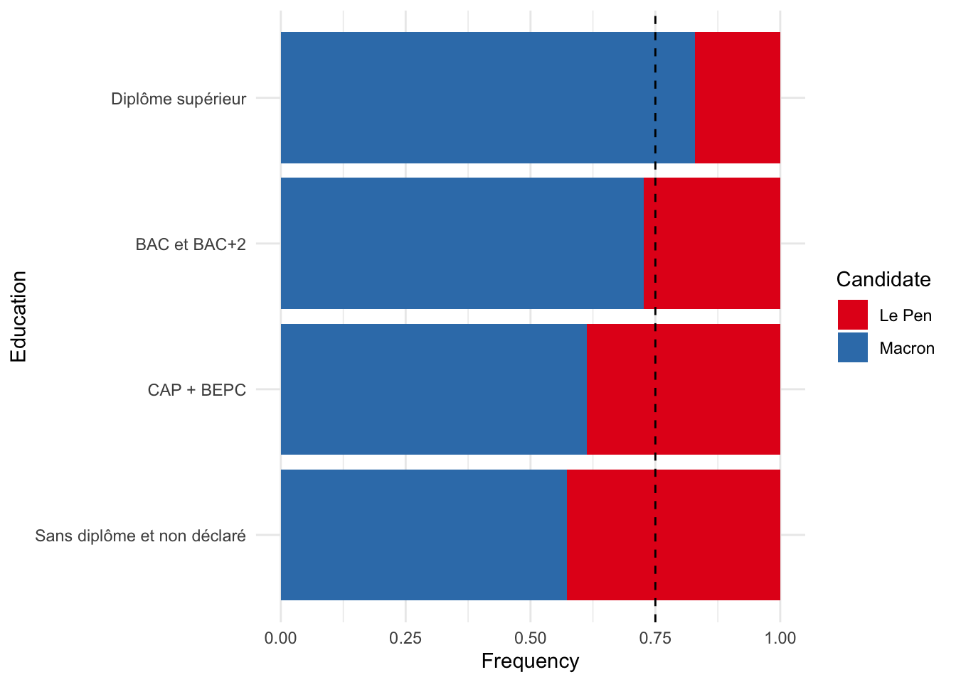
From this table, we can already see that the vote choice vary across education level. The total col shows us what would be the distribution of voting choice if there was no relationship between education and voting choice. But we can see that voters with higher education have voted more for Macron than for Le Pen.
But is this difference statistically significant ? To answer this question, we can use a χ² test that will tell us if the observed distribution is different from the expected distribution. To do this in R, we can use the chisq.test() function.
(test_educ <- chisq.test(fes2022$candidate_t2, fes2022$education))
    Pearson's Chi-squared test

data:  fes2022$candidate_t2 and fes2022$education
X-squared = 54.705, df = 3, p-value = 7.936e-12
test_educ
    Pearson's Chi-squared test

data:  fes2022$candidate_t2 and fes2022$education
X-squared = 54.705, df = 3, p-value = 7.936e-12
This gives us three informations :
- The X-squared value, which is our test statistic. It is computed by comparing the observed values to the expected values. You can access them with
test_educ$statistic.ithbroom::augment(). Expected values are the values that we would expect if there was no relationship between the two variables. The test is computed by comparing the observed values to the expected values.
(augmented <- augment(test_educ)) |> select(1:3, 7) |> view()The degrees of freedom (3) that is computed by
df = (number of rows - 1) * (number of columns - 1). Here :(2-1)*(4-1).Our p-value set at a critical value of 0.05. The p-value is the probability of observing a test statistic as extreme or more extreme than the one we observed if the null hypothesis is true. Based on this critical value and the X-squared value, the chi2 table gives us that p-value. Here, the p-value is 7.936e-12, which is equivalent to 0.000000000007936. Our result mean that the chance we reject a true null hypothesis is 7.936e-12. So we can reject the null hypothesis and conclude that there is a statistically significant relationship between education and voting choice.
We can also use the tidy() function from broom to get the results in a tibble.
test_educ |>
  tidy() |>  # Get the results in a tibble
  mutate(is_significant = p.value < 0.05) # Add a column to see if the result is significant
# A tibble: 1 × 5
statistic p.value parameter method is_significant
<dbl> <dbl> <int> <chr> <lgl>
1 54.7 7.94e-12 3 Pearson's Chi-squared test TRUE We can also look at the residuals. The residuals are the difference between the observed and the expected values. They are standardized by the expected values. So, if the residual is positive, it means that the observed value is higher than the expected value. If the residual is negative, it means that the observed value is lower than the expected value.
augmented |>
  select(fes2022.candidate_t2, fes2022.education, .resid) |>
  arrange(- .resid) # Arrange the residuals in descending order
# A tibble: 8 × 3
fes2022.candidate_t2 fes2022.education .resid
<fct> <fct> <dbl>
1 Le Pen CAP + BEPC 4.14
2 Le Pen Sans diplôme et non déclaré 2.90
3 Macron Diplôme supérieur 2.25
4 Le Pen BAC et BAC+2 0.615
5 Macron BAC et BAC+2 -0.356
6 Macron Sans diplôme et non déclaré -1.68
7 Macron CAP + BEPC -2.39
8 Le Pen Diplôme supérieur -3.89 Using the infer package, we can also visualize how far is our observed statistic from the distribution of statistics under the null hypothesis.
# calculate the observed statistic
observed_indep_statistic <- fes2022 |>
  drop_na(candidate_t2) |>
  specify(candidate_t2 ~ education) |>
  hypothesize(null = "independence") |>
  calculate(stat = "Chisq")

observed_indep_statistic
Response: candidate_t2 (factor)
Explanatory: education (factor)
Null Hypothesis: independence
# A tibble: 1 × 1
stat
<dbl>
1 54.7# calculate the null distribution
null_dist_sim <- fes2022 |>
drop_na(candidate_t2) |>
specify(candidate_t2 ~ education) |>
hypothesize(null = "independence") |>
generate(reps = 1000, type = "permute") |>
calculate(stat = "Chisq")
# Visualize the null distribution and shade the observed statistic
null_dist_sim |>
visualize() +
shade_p_value(observed_indep_statistic,
direction = "greater")Warning in min(diff(unique_loc)): no non-missing arguments to min; returning
Inf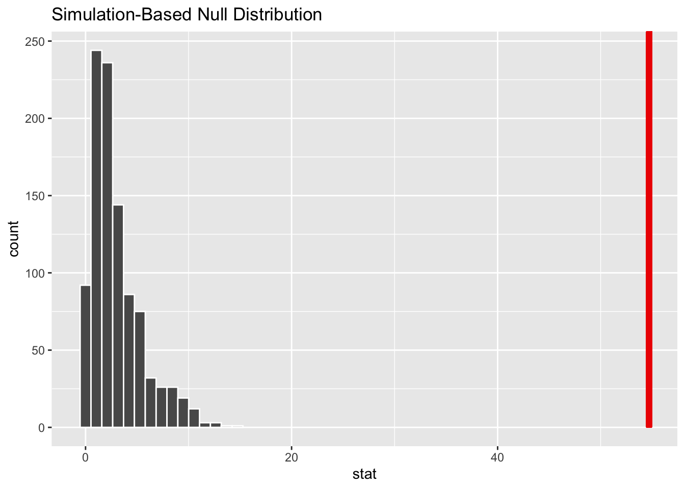
12.6 Relationship between a categorical and a continuous variable : t-test
Thus far, we have examined the relationship between two categorical variables. However, there are instances when we are interested in assessing how various groups vary in terms of their values on a continuous variable. For this, we can use a t-test, which is a statistical test that allows us to compare the means of two groups. The t-test is used to test the null hypothesis that there is no difference between the means of the two groups. The alternative hypothesis is that there is a difference between the means of the two groups. Our goal is to reject the null hypothesis.
Here, I want to know if voters of Macron and Le Pen during the second round of the election differ in their level of political trust.
H0 : There is no difference between voting choice and political trust H1 : There is a difference between voting choice and political trust
In our dataset, we have various trust-related variables. I’m particularly interested in political trust, which includes three specific variables: trust in parliament, trust in government, and trust in political parties.
view(variables)
variables |> filter(str_detect(label, "Confiance"))
# A tibble: 7 × 3
variable label categories
<chr> <chr> <chr>
1 fes4_Q07a Confiance : - Parlement `Tout à fait confiance` = 1, `Pl…
2 fes4_Q07b Confiance : - Gouvernement `Tout à fait confiance` = 1, `Pl…
3 fes4_Q07d Confiance : - Scientifiques `Tout à fait confiance` = 1, `Pl…
4 fes4_Q07e Confiance : - Partis politiques `Tout à fait confiance` = 1, `Pl…
5 fes4_Q07f Confiance : - Médias Traditionnels `Tout à fait confiance` = 1, `Pl…
6 fes4_Q07g Confiance : - Réseaux Sociaux `Tout à fait confiance` = 1, `Pl…
7 eayy_f9 Confiance de manière générale `0 - On n'est jamais assez prude…# Compute the mean of the fes4_q07 variables
fes2022 |>
summarise(across(c(fes4_Q07a, fes4_Q07b, fes4_Q07e), ~ mean(.x, na.rm = TRUE)))# A tibble: 1 × 3
fes4_Q07a fes4_Q07b fes4_Q07e
<dbl> <dbl> <dbl>
1 2.40 2.61 3.01To have a summary of these three variables, I can create a composite index by adding the sum of these three variables. To be more robust, I should also test how these variables correlate with each other. But this is beyond the scope of this course so I just add them together. I can also standardize this index and rescale it between 1 and 0. This also reverse the scale of the index, so that a higher value means a higher level of trust.
fes2022 |>
  count(fes4_Q07a)
# A tibble: 5 × 2
fes4_Q07a n
<dbl+lbl> <int>
1 1 [Tout à fait confiance] 59
2 2 [Plutôt confiance] 943
3 3 [Plutôt pas confiance] 446
4 4 [Pas du tout confiance] 119
5 NA(a) 8# Create a trust index computing the sum of different trust variables
fes2022 <- fes2022 |>
mutate(
trust_index = fes4_Q07a + fes4_Q07b + fes4_Q07e,
trust_index2 = scales::rescale(trust_index, to = c(1, 0)))
fes2022 |> count(trust_index)# A tibble: 11 × 2
trust_index n
<dbl> <int>
1 3 2
2 4 10
3 5 25
4 6 237
5 7 463
6 8 258
7 9 264
8 10 145
9 11 74
10 12 80
11 NA 17fes2022 |> count(trust_index2)# A tibble: 11 × 2
trust_index2 n
<dbl> <int>
1 0 80
2 0.111 74
3 0.222 145
4 0.333 264
5 0.444 258
6 0.556 463
7 0.667 237
8 0.778 25
9 0.889 10
10 1 2
11 NA 17fes2022 |> count(candidate_t2)# A tibble: 3 × 2
candidate_t2 n
<chr> <int>
1 Le Pen 270
2 Macron 808
3 <NA> 497Now let’s have a look on how voters of our two candidates differ in terms of their level of trust. We can see that the difference is quite clear. Voters of Macron have much more higher level of trust than voters of Le Pen.
# Look at how groups differ in terms of trust
fes2022 |>
  group_by(candidate_t2) |>
  summarise(trust_index = mean(trust_index2, na.rm = TRUE))
# A tibble: 3 × 2
candidate_t2 trust_index
<chr> <dbl>
1 Le Pen 0.303
2 Macron 0.529
3 <NA> 0.376# Look at this visually
fes2022 |>
ggplot(aes(x = candidate_t2, y = trust_index2)) +
geom_boxplot()Warning: Removed 17 rows containing non-finite values (`stat_boxplot()`).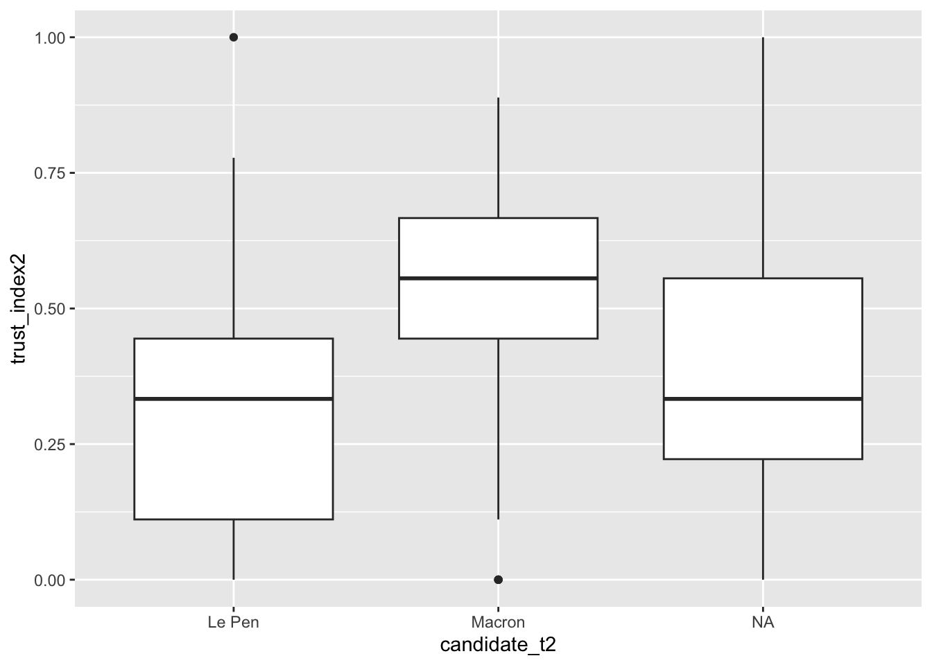
We can test this statistically by using a t.test that will tell us if the difference between the two groups is statistically significant. To do so, we use the t.test() function that takes as input the two variables we want to compare with a ~ in between and the data where it comes from. Here, we want to compare the level of trust between voters of Macron and Le Pen. So, we use the trust_index2 variable as the first argument and the candidate_t2 variable as the second argument. We also specify the dataset we want to use with the data argument.
(test <- t.test(fes2022$trust_index2 ~ fes2022$candidate_t2))
    Welch Two Sample t-test

data:  fes2022$trust_index2 by fes2022$candidate_t2
t = -16.881, df = 353.99, p-value < 2.2e-16
alternative hypothesis: true difference in means between group Le Pen and group Macron is not equal to 0
95 percent confidence interval:
 -0.2524035 -0.1997278
sample estimates:
mean in group Le Pen mean in group Macron
           0.3030680            0.5291336
(test <- t.test(trust_index2 ~ candidate_t2, data = fes2022))
    Welch Two Sample t-test

data:  trust_index2 by candidate_t2
t = -16.881, df = 353.99, p-value < 2.2e-16
alternative hypothesis: true difference in means between group Le Pen and group Macron is not equal to 0
95 percent confidence interval:
 -0.2524035 -0.1997278
sample estimates:
mean in group Le Pen mean in group Macron
           0.3030680            0.5291336
The results of the test show us that the difference between the two groups is statistically significant. The alternative hypothesis is that the difference between the two groups is not equal to 0. The p-value is lower than 0.05, so we can reject the null hypothesis. There is a relationship between the candidate voted for and the level of trust.
We can also use the tidy() function from broom to get the results in a tibble.
test |>
  tidy()
# A tibble: 1 × 10
estimate estimate1 estimate2 statistic p.value parameter conf.low conf.high
<dbl> <dbl> <dbl> <dbl> <dbl> <dbl> <dbl> <dbl>
1 -0.226 0.303 0.529 -16.9 2.55e-47 354. -0.252 -0.200
# ℹ 2 more variables: method <chr>, alternative <chr>test |>
tidy() |>
mutate(is_significant = p.value < 0.05) |>
select(p.value, is_significant)# A tibble: 1 × 2
p.value is_significant
<dbl> <lgl>
1 2.55e-47 TRUE