# Import packages

needs(tidyverse, janitor, labelled, broom, haven)

# Import ess data

ess <- haven::read_dta("data/ess8.dta")

n_distinct(ess$cntry) # 23 different countries
[1] 23In practice, linear regression is rarely performed with only one variable but instead with multiple variables. The purpose of using multiple variables is not solely to understand the effect of one variable on another, but rather to “isolate” this effect by controlling for other independent variables that may also contribute to explaining the variance of the dependent variable. This concept is commonly known as ceteris paribus, which means keeping all other factors constant.
In R, to conduct a linear regression while controlling for multiple independent variables, you can use the lm() function and specify the formula as follows: lm(y ~ x + z + w, data). In this formula, y represents the dependent variable, while x, z, and w represent the independent variables you want to include in the model. The data argument is used to specify the dataset from which the variables are taken.
To learn how to conduct multiple regression in R, we will work with the European Social Survey. We will investigate the question of the gender gap in climate policy attitudes. Is there any gender difference in the way people support climate policies? Part of the literature (Bush and Clayton 2023) suggests this, and we want to test whether it is true using European Social Survey data and examine how this varies across countries. Here I use the 8th wave of the ESS that contains variables on climate policy support.
# Import packages
needs(tidyverse, janitor, labelled, broom, haven)
# Import ess data
ess <- haven::read_dta("data/ess8.dta")
n_distinct(ess$cntry) # 23 different countries[1] 23To assess the effect of gender of climate policy support, I rely on three different variables that are in the dataset :
banhhap : “Favour ban sale of least energy efficient household appliances to reduce climate change”inctxff : “Favour increase taxes on fossil fuels to reduce climate change”sbsrnen : “Favour subsidies for renewable energy to reduce climate change”# A look at the variables labels
ess |>
select(banhhap, inctxff, sbsrnen) |>
map(var_label)$banhhap
[1] "Favour ban sale of least energy efficient household appliances to reduce climate"
$inctxff
[1] "Favour increase taxes on fossil fuels to reduce climate change"
$sbsrnen
[1] "Favour subsidise renewable energy to reduce climate change"Each of the variables is coded from 1 to 5, where 1 means “Strongly in favour” and 5 means “Strongly against”. Hence, the higher the value, the more people are against climate policies.
# A look at the different categories

ess |>
  select(banhhap, inctxff, sbsrnen) |>
  map(val_labels)
$banhhap
Strongly in favour Somewhat in favour
1 2
Neither in favour nor against Somewhat against
3 4
Strongly against Refusal
5 NA
Don't know No answer
NA NA
$inctxff
Strongly in favour Somewhat in favour
1 2
Neither in favour nor against Somewhat against
3 4
Strongly against Refusal
5 NA
Don't know No answer
NA NA
$sbsrnen
Strongly in favour Somewhat in favour
1 2
Neither in favour nor against Somewhat against
3 4
Strongly against Refusal
5 NA
Don't know No answer
NA NA Before starting, it is always good to have a look at the distribution of the variables. From the distribution, we can see that the patterns of opposition to climate policies are different across the three variables. People tend to support more subsidies for renewable energy, and the ban of least energy efficient household appliances. The support for increasing taxes on fossil fuels is the lowest and is more dispersed.
# Create histogram for each of the variables

ess |>
  select(banhhap, inctxff, sbsrnen) |>
  # Convert to long format
  pivot_longer(everything(), names_to = "policy", values_to = "opposition") |>
  ggplot(aes(opposition)) +
  geom_bar() +
  facet_wrap(~policy)
Warning: Removed 5078 rows containing non-finite values (`stat_count()`).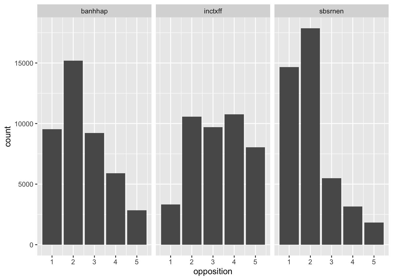
Before running a regression, we need to recode the variables of interest. My main independent variable is gender but I also control for other important variables that might influence climate policy support such as left-right self-placement (lrscale), education (eduyrs), income (hincfel), age (yrbrn) and satisfaction with the economic situation (stfeco).
# Recode gender

ess |>
  count(gndr)
# A tibble: 3 × 2
gndr n
<dbl+lbl> <int>
1 1 [Male] 21027
2 2 [Female] 23351
3 NA(a) [No answer] 9ess <- ess |>
mutate(gender = unlabelled(gndr) |> as_factor())
ess |>
count(gender)# A tibble: 3 × 2
gender n
<fct> <int>
1 Male 21027
2 Female 23351
3 <NA> 9# Recode independent variables
## Recode left-right and satisfaction with the economic situation
ess |>
count(lrscale)# A tibble: 12 × 2
lrscale n
<dbl+lbl> <int>
1 0 [Left] 1463
2 1 [1] 846
3 2 [2] 2121
4 3 [3] 3754
5 4 [4] 3780
6 5 [5] 12389
7 6 [6] 4105
8 7 [7] 4269
9 8 [8] 3265
10 9 [9] 999
11 10 [Right] 1592
12 NA(b) [Don't know] 5804ess <- ess |>
mutate(
left_right = case_when(
# when lrscale is NA, replace with the mean of the variable
is.na(lrscale) ~ mean(lrscale, na.rm = TRUE),
# otherwise, keep the value of the variable
TRUE ~ lrscale
),
stfeco = case_when(
# when stfeco is NA, replace with the mean of the variable
is.na(stfeco) ~ mean(stfeco, na.rm = TRUE),
# otherwise, keep the value of the variable
TRUE ~ stfeco |> as.integer()
),
# create index of political trust
)
## Recode income, age and education
ess |>
count(eduyrs)# A tibble: 43 × 2
eduyrs n
<dbl+lbl> <int>
1 0 97
2 1 38
3 2 58
4 3 161
5 4 428
6 5 442
7 6 443
8 7 659
9 8 2491
10 9 2319
# ℹ 33 more rowsess <- ess |>
mutate(
# Transform year of birth into age
age = 2016 - yrbrn
)# Add index of political trust with PCA
ess |>
select(starts_with("trst")) |>
map(var_label)$trstlgl
[1] "Trust in the legal system"
$trstplc
[1] "Trust in the police"
$trstplt
[1] "Trust in politicians"
$trstep
[1] "Trust in the European Parliament"
$trstun
[1] "Trust in the United Nations"
$trstprt
[1] "Trust in political parties"
$trstprl
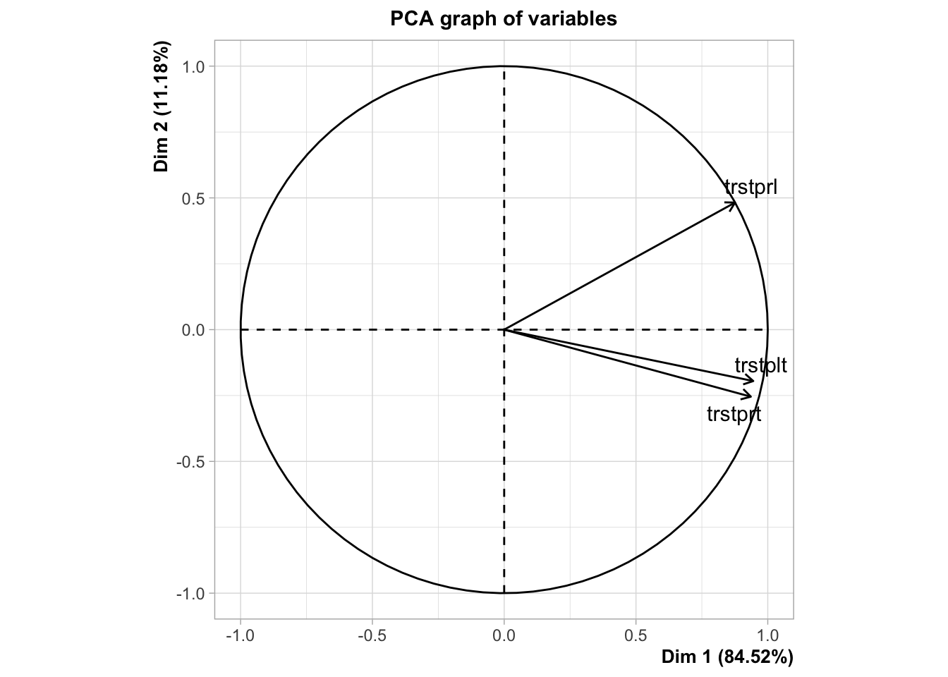
[1] "Trust in country's parliament"pca_trust <- ess |>
# Select main variables of political trust
select(trstprl, trstprt, trstplt) |>
# Run PCA on them
FactoMineR::PCA(scale.unit = T) |>
# Extract the coordinates of the different dimensions
pluck("ind", "coord") |>
# Convert it into a tibble
as_tibble() |>
# Keep only the first dimension
select(1) |>
# Rename it to trust index
rename(trust_index = Dim.1) Warning in FactoMineR::PCA(select(ess, trstprl, trstprt, trstplt), scale.unit =
T): Missing values are imputed by the mean of the variable: you should use the
imputePCA function of the missMDA package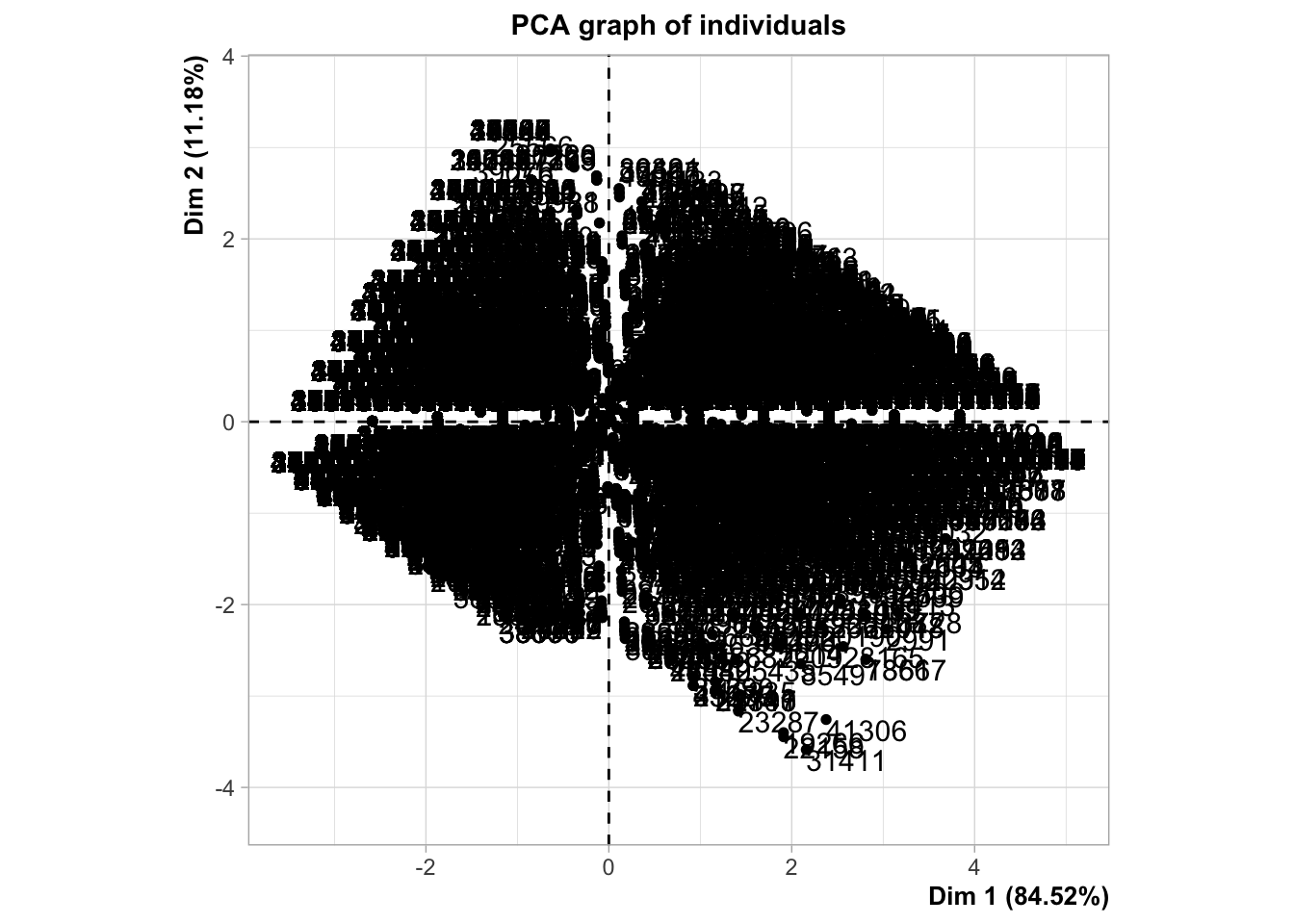
ess <- bind_cols(ess, pca_trust) # Add the index to the dataset

ess |>
  ggplot(aes(trust_index)) +
  geom_histogram()
`stat_bin()` using `bins = 30`. Pick better value with `binwidth`.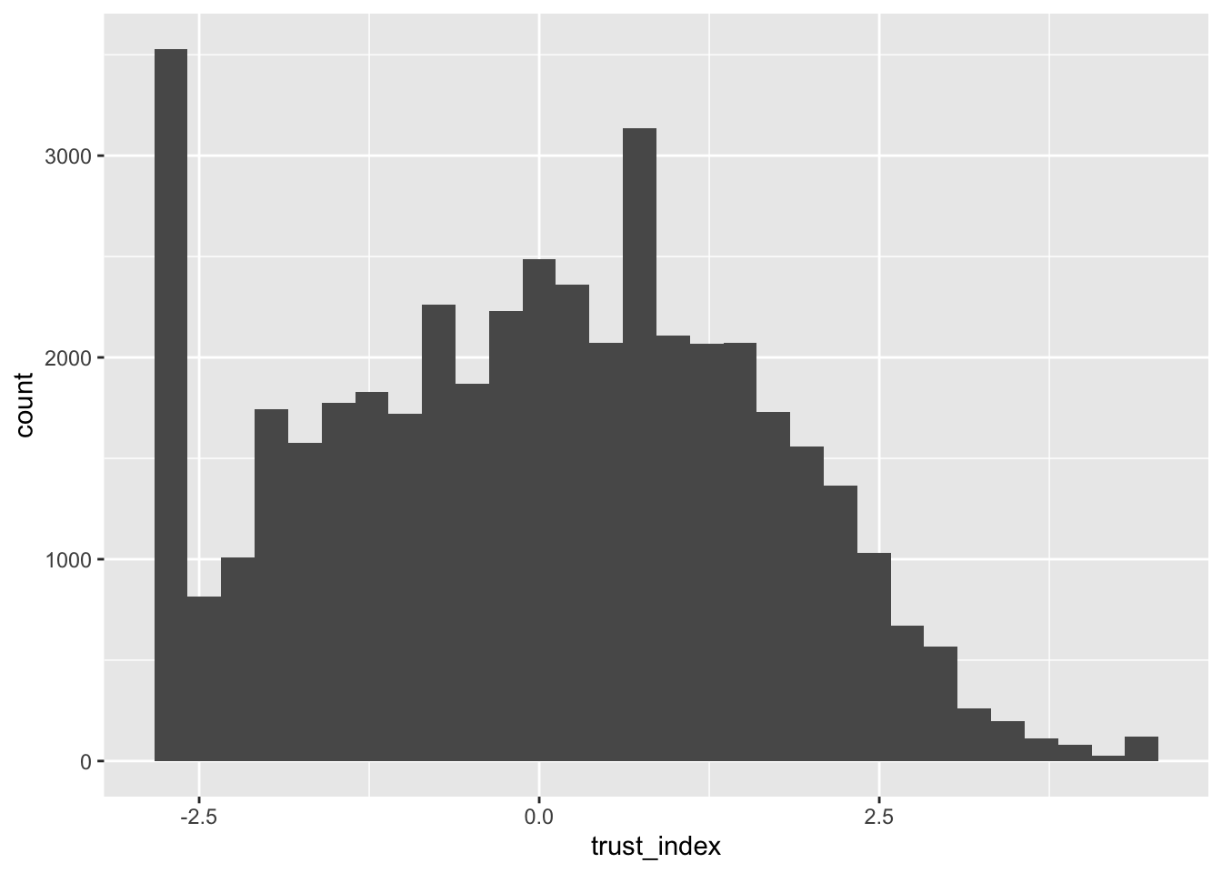
model1 <- lm(sbsrnen ~ gender + eduyrs + hincfel + left_right + age  + stfeco + trust_index, ess)

model2 <- lm(inctxff ~ gender + eduyrs + hincfel + left_right  + age  + stfeco + trust_index, ess)

model3 <- lm(banhhap~ gender + eduyrs + left_right + hincfel + age + stfeco + trust_index, ess)stargazer::stargazer(model1, model2, model3,
title = "Model Results",
align = TRUE,
type = "text",
dep.var.labels = "Climate policy opposition",
covariate.labels = c("Gender")
) Dependent variable:
-------------------------------------------------------------------------------
Climate policy opposition inctxff banhhap
(1) (2) (3) | Gender -0.042*** -0.055*** -0.097*** (0.010) (0.012) (0.011) |
|---|
| Observations 42,130 41,588 41,861 R2 0.022 0.083 0.012 Adjusted R2 0.022 0.083 0.012 Residual Std. Error 1.053 (df = 42122) 1.183 (df = 41580) 1.162 (df = 41853) F Statistic 136.471*** (df = 7; 42122) 537.033*** (df = 7; 41580) 75.217*** (df = 7; 41853) =================================================================================================== Note: p<0.1; p<0.05; p<0.01 |
| ## PLotting the coefficeints |
| When we have different variables : useful to plot the different coefficients. |
| - You can extract the outputs of model with broom and use them to plot the results - Interpretation for categorical : do not forget refernce |
| ::: {.cell} |
| ```{.r .cell-code} # Plot the coefficients of the model models_coefficients <- map_df(list(model1, model2, model3), ~ tidy(.x, conf.int = T), .id = “model”) |
| models_coefficients |> filter(term != “(Intercept)”) |> ggplot(aes(term, estimate, color = model)) + geom_pointrange(aes(ymin = conf.low, ymax = conf.high), position = position_dodge(width = 0.5)) + geom_hline(yintercept = 0, linetype = “dashed”) + coord_flip() + labs(x = “Coefficient”, y = NULL, title = “Coefficients of the different models”) + theme_minimal() + scale_color_manual(labels = c(“Subsidies”, “Tax”, “Ban”), values = c(“#00AFBB”, “#E7B800”, “#FC4E07”)) ``` |
::: {.cell-output-display} 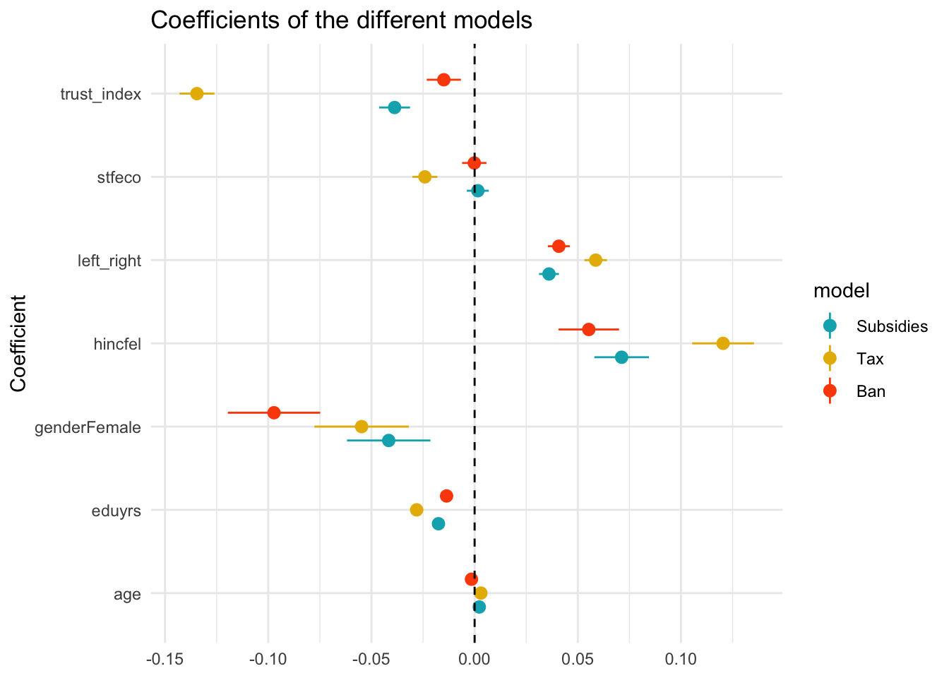 ::: ::: ::: ::: |
| ## Predicted values of the model |
| ::: {.cell} |
{.r .cell-code} ggeffects::ggpredict(model2, terms = "gender") |
| ::: {.cell-output .cell-output-stdout} ``` # Predicted values of Favour increase taxes on fossil fuels to reduce climate change |
| gender | Predicted | 95% CI |
Male | 3.25 | [3.24, 3.27] Female | 3.20 | [3.18, 3.21]
Adjusted for: * eduyrs = 13.12 * hincfel = 1.93 * left_right = 5.15 * age = 48.67 * stfeco = 5.07 * trust_index = 0.03
:::

```{.r .cell-code}
ggeffects::ggpredict(model2, terms = "gender") |>
  plot() +
  ggtitle("Opposition to tax") +
  ylab("Opposition to tax")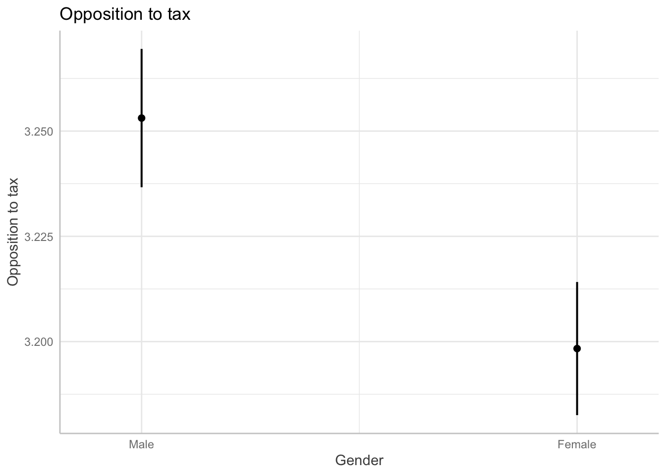
:::
model4 <- lm(inctxff ~ gender*left_right + eduyrs + hincfel+ age  + stfeco + trust_index, ess)

stargazer::stargazer(model4, type = "text")
===================================================
                            Dependent variable:
                        ---------------------------
                                  inctxff
---------------------------------------------------
genderFemale                      -0.006
                                  (0.031)

left_right                       0.063***
                                  (0.004)

eduyrs                           -0.028***
                                  (0.002)

hincfel                          0.121***
                                  (0.008)

age                              0.003***
                                 (0.0003)

stfeco                           -0.024***
                                  (0.003)

trust_index                      -0.134***
                                  (0.004)

genderFemale:left_right           -0.009*
                                  (0.006)

Constant                         3.041***
                                  (0.045)

---------------------------------------------------
Observations                      41,588
R2                                 0.083
Adjusted R2                        0.083
Residual Std. Error         1.183 (df = 41579)
F Statistic             470.286*** (df = 8; 41579)
===================================================
Note: *p<0.1; **p<0.05; ***p<0.01ggeffects::ggpredict(model4, terms = c("left_right", "gender")) |>
as_tibble() |>
ggplot(aes(x, predicted, color = group)) +
geom_line() +
geom_ribbon(aes(ymin = conf.low, ymax = conf.high), alpha = 0.2)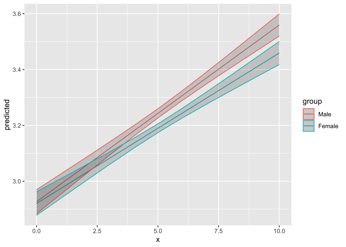
Once we’ve fit our model, however, we need to perform several diagnostics to see if the specification is right and if we’re not breaking various underlying assumptions we make about the data when we use regression. Here, we use the performance package to check different of these assumptions.
needs(performance)vif() function from the car package.If it’s useful to check for collinearity, be aware that the extent to which this is an important issue is open to debate. For instance, see the takes of Paul Allison and Richard McElreath.
One way in R to check for multicolinearity is from the check_collinearity() function from the performance package (equivalent to the car::vif function). The functions calculate the VIF, give confidence interval and calculte tolerance.
map(list(model1, model2, model3), check_collinearity)[[1]]
# Check for Multicollinearity
Low Correlation
Term VIF VIF 95% CI Increased SE Tolerance Tolerance 95% CI
gender 1.01 [1.00, 1.03] 1.00 0.99 [0.97, 1.00]
eduyrs 1.12 [1.11, 1.13] 1.06 0.89 [0.88, 0.90]
hincfel 1.18 [1.16, 1.19] 1.08 0.85 [0.84, 0.86]
left_right 1.02 [1.01, 1.03] 1.01 0.98 [0.97, 0.99]
age 1.05 [1.04, 1.06] 1.03 0.95 [0.94, 0.96]
stfeco 1.46 [1.44, 1.48] 1.21 0.68 [0.68, 0.69]
trust_index 1.39 [1.37, 1.41] 1.18 0.72 [0.71, 0.73]
[[2]]
# Check for Multicollinearity
Low Correlation
Term VIF VIF 95% CI Increased SE Tolerance Tolerance 95% CI
gender 1.01 [1.00, 1.03] 1.00 0.99 [0.97, 1.00]
eduyrs 1.12 [1.11, 1.14] 1.06 0.89 [0.88, 0.90]
hincfel 1.18 [1.16, 1.19] 1.08 0.85 [0.84, 0.86]
left_right 1.02 [1.01, 1.03] 1.01 0.98 [0.97, 0.99]
age 1.05 [1.04, 1.06] 1.03 0.95 [0.94, 0.96]
stfeco 1.46 [1.45, 1.48] 1.21 0.68 [0.67, 0.69]
trust_index 1.39 [1.38, 1.41] 1.18 0.72 [0.71, 0.73]
[[3]]
# Check for Multicollinearity
Low Correlation
Term VIF VIF 95% CI Increased SE Tolerance Tolerance 95% CI
gender 1.01 [1.00, 1.03] 1.00 0.99 [0.97, 1.00]
eduyrs 1.12 [1.11, 1.13] 1.06 0.89 [0.88, 0.90]
left_right 1.02 [1.01, 1.03] 1.01 0.98 [0.97, 0.99]
hincfel 1.18 [1.17, 1.19] 1.09 0.85 [0.84, 0.86]
age 1.05 [1.04, 1.06] 1.03 0.95 [0.94, 0.96]
stfeco 1.46 [1.44, 1.48] 1.21 0.68 [0.68, 0.69]
trust_index 1.39 [1.37, 1.41] 1.18 0.72 [0.71, 0.73]check_heteroscedasticity(model2) Warning: Heteroscedasticity (non-constant error variance) detected (p < .001).To detect outliers, we use the cook distance which is an outlier detection methods. It estimate how much our regression coefficients change if we remove each observation.
check_outliers(model1)OK: No outliers detected.
- Based on the following method and threshold: cook (0.907).
- For variable: (Whole model)purrrLet’s say I want to know how our estimates would be different for different policies but also for different countries.
n_distinct(ess$cntry) # 23 different countries[1] 23ess_models <- ess |>
# Select variables of interest
select(cntry,
gender,
left_right,
hincfel,
age,
trust_index,
eduyrs,
inctxff,
banhhap,
sbsrnen,
stfeco) |>
# Pivot longer to have one column for the policy and one for the values for each respondent
pivot_longer(
cols = c(inctxff, banhhap, sbsrnen),
names_to = "policy",
values_to = "opposition")
ess_models <- ess_models |>
# Nest the data by country and policy
nest(data = -c(cntry, policy))
ess_models <- ess_models |>
mutate(
# For each country-policy pairs, fit a model
model = map(
data,
~ lm(opposition ~ gender + left_right + hincfel + age + eduyrs + stfeco + trust_index, .x)
),
# Extract the coefficients of each model in a tidied column
tidied = map(model, ~ tidy(.x, conf.int = T)),
# Extract the R2 of each model in a glanced column
glanced = map(model, glance),
# Extract the residuals of each model in a augmented column
augmented = map(model, augment)
)
ess_models# A tibble: 69 × 7
cntry policy data model tidied glanced augmented
<chr> <chr> <list> <list> <list> <list> <list>
1 AT inctxff <tibble [2,010 × 8]> <lm> <tibble [8 × 7]> <tibble> <tibble>
2 AT banhhap <tibble [2,010 × 8]> <lm> <tibble [8 × 7]> <tibble> <tibble>
3 AT sbsrnen <tibble [2,010 × 8]> <lm> <tibble [8 × 7]> <tibble> <tibble>
4 BE inctxff <tibble [1,766 × 8]> <lm> <tibble [8 × 7]> <tibble> <tibble>
5 BE banhhap <tibble [1,766 × 8]> <lm> <tibble [8 × 7]> <tibble> <tibble>
6 BE sbsrnen <tibble [1,766 × 8]> <lm> <tibble [8 × 7]> <tibble> <tibble>
7 CH inctxff <tibble [1,525 × 8]> <lm> <tibble [8 × 7]> <tibble> <tibble>
8 CH banhhap <tibble [1,525 × 8]> <lm> <tibble [8 × 7]> <tibble> <tibble>
9 CH sbsrnen <tibble [1,525 × 8]> <lm> <tibble [8 × 7]> <tibble> <tibble>
10 CZ inctxff <tibble [2,269 × 8]> <lm> <tibble [8 × 7]> <tibble> <tibble>
# ℹ 59 more rowsThe coefficient plot will give us an estimate of the effect of gender of each of the three policy for each country. We can see that there is some heterogeneity and that the gender effect is not always significant.
ess_models |>
  # Unnest the dataset
  unnest(tidied) |>
  # Filter to keep only the coefficient of interest
  filter(term == "genderFemale") |>
  # Create a column to indicate if the coefficient is significant
  mutate(significant = p.value < 0.05) |>
  # Create a coefficient plot for each country and policy
  ggplot(aes(fct_reorder(cntry, estimate), estimate, color = significant)) +
  geom_pointrange(aes(ymin = conf.low, ymax = conf.high), position = position_dodge(width = 1)) +
  coord_flip() +
  geom_hline(yintercept = 0, linetype = "dashed") +
  theme_light() +
  labs(x = "Country") +
  facet_wrap(~ policy) +
  scale_colour_viridis_d()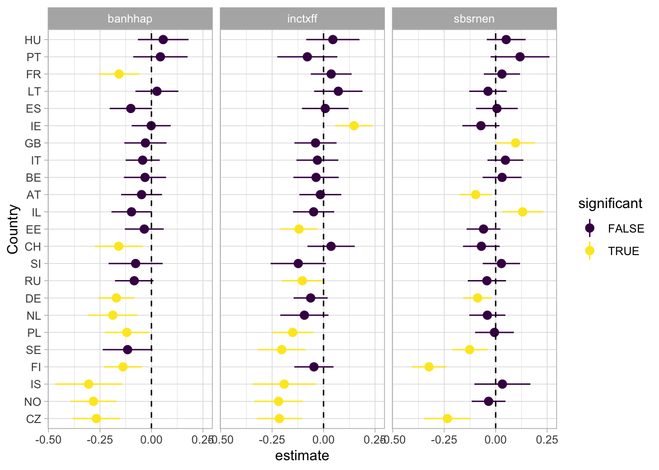
If we look at the results of our estimate for the left-right variable, the results are even more clear. We tend to see a divide between eastern and western european countries.
ess_models |>
  unnest(tidied) |>
  filter(term == "left_right") |>
  mutate(
    significant = p.value > 0.05,
    policy = case_match(
      policy,
      "banhhap" ~ "Ban sale non efficient households",
      "inctxff" ~ "Tax fossil fuels",
      "sbsrnen" ~ "Subsidies renewable"
    )
  ) |>
  ggplot(aes(fct_reorder(cntry, estimate), estimate, color = significant)) +
  geom_pointrange(aes(ymin = conf.low, ymax = conf.high), position = position_dodge(width = 1)) +
  coord_flip() +
  geom_hline(yintercept = 0, linetype = "dashed") +
  theme_light() +
  labs(x = "Country") +
  scale_colour_viridis_d() +
  facet_wrap( ~ policy)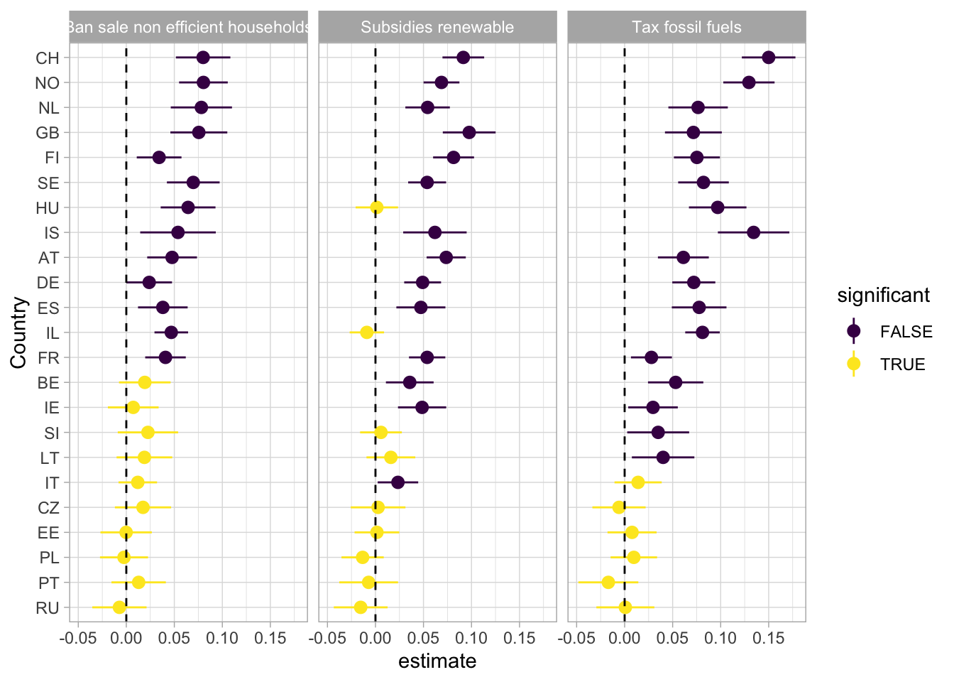
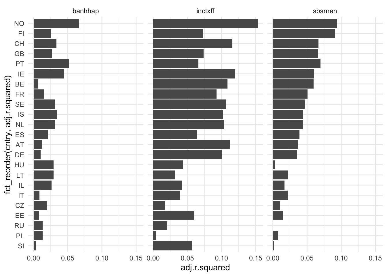
ess_models |>
  unnest(glanced) |>
  ggplot(aes(fct_reorder(cntry, adj.r.squared), adj.r.squared)) +
  geom_col() +
  coord_flip() +
  facet_wrap(~ policy) +
  theme_minimal()