As you may have learned in your quantitative methods class, correlation often falls short, and linear regression is frequently employed. Linear regression is considered a workhorse in quantitative social sciences. It’s safe to say that publishing quantitative results can be challenging without utilizing this or a more sophisticated model. Whether you’re a quantitative researcher aiming to employ it or a qualitative researcher seeking to comprehend a quantitative article relevant to your work, understanding how regression operates is crucial.
When dealing with a sole dependent variable, we refer to it as simple linear regression, which is our primary focus today. In the next session, we will delve into multiple linear regression, involving more than one independent variable.
In linear regression, our objective is to establish a linear relationship between one or more independent variables and a continuous dependent variable. However, when working with a dependent variable that is not continuous, other models become relevant, and these will be explored in the upcoming semester. One such model is logistic regression, which is employed when the dependent variable is binary (e.g., whether individuals have voted for Trump or not).
14.1 Testing economic voting theory
To understand how it works, I am using an example developed by François Briatte, the previous instructor of this course, which utilizes data from Larry Bartels on economic voting in the United States. Economic voting is a theory that suggests voters reward or punish the incumbent government based on the state of the economy. In this example, we will explore the relationship between changes in real disposable income in the last quarters before an election and the margin of victory for the incumbent party in the United States.
Our question is then : Is there a relationship between the state of the economy (measured as the growth of real disponible income) and the margin of victory for the incumbent party in the United States? Our regression equation for each incumbent party is a given year \({i}\) is written below.
\[
margin_{i} = \beta_{0} + \beta_{1}income_{i} + \epsilon_{i}
\] The goal of the regression is to estimate the parameters of our model wich are \(\beta_{0}\), \(\beta_{1}\) and \(\epsilon_{i}\).
\(\beta_{0}\) corresponds to the intercept of the regression line. It provides the estimated value of the margin of victory for the incumbent party when the growth of real disposable income is 0. This intercept may or may not have a meaningful interpretation depending on the context of your data.
\(\beta_{1}\) represents the slope of the regression line. It indicates the estimated change in the margin of victory for the incumbent party for a one-unit change in the growth of real disposable income. This coefficient is of particular interest as it demonstrates the strength and direction of the relationship between the two variables.
\(\epsilon_{i}\) is the error term
To estimate the parameters of our model, we use the method of ordinary least squares (OLS). It allows to fit a line through the data points in a way that minimizes the sum of the squared prediction errors. In other words, it minimizes the distance between the line and the data points. This is why it is called “least squares”. This might still sound abstract to you so let’s look at the data ! I first import the data that is in two datasets that I am merging together.
# Import the packagesneeds(tidyverse, broom, stargazer)# Import the two datasetsbartels <-read_csv("data/bartels4812.csv")
Rows: 17 Columns: 5
── Column specification ────────────────────────────────────────────────────────
Delimiter: ","
dbl (5): year, incm, tenure, inc1415, rdpic

ℹ Use `spec()` to retrieve the full column specification for this data.
ℹ Specify the column types or set `show_col_types = FALSE` to quiet this message.
Rows: 19 Columns: 6
── Column specification ────────────────────────────────────────────────────────
Delimiter: ","
chr (3): president, party, challenger
dbl (3): year, incumbent, unelected

ℹ Use `spec()` to retrieve the full column specification for this data.
ℹ Specify the column types or set `show_col_types = FALSE` to quiet this message.
# Join them togetherelec <-left_join(bartels, presidents, by ="year")
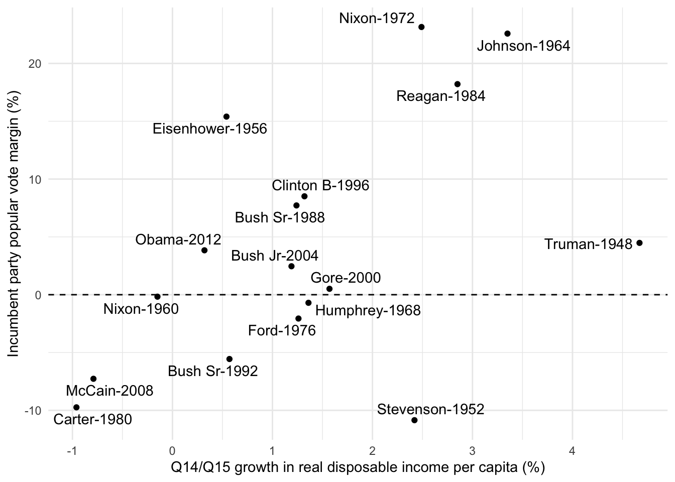
To explore the relationship between the two variables, we first draw a scatter plot. We see from this plot that there seems to be a linear relationship.
(elec_plot <- elec |>ggplot(aes(inc1415, incm)) +# Create a scatter plotgeom_point() +# Add a line at 0 on the y-axisgeom_hline(yintercept =0, lty ="dashed") +# Add president names ggrepel::geom_text_repel(aes(label =str_c(incumbent, "-", year))) +# Change axix labelslabs(y ="Incumbent party popular vote margin (%)",x ="Q14/Q15 growth in real disposable income per capita (%)" ) +theme_minimal())
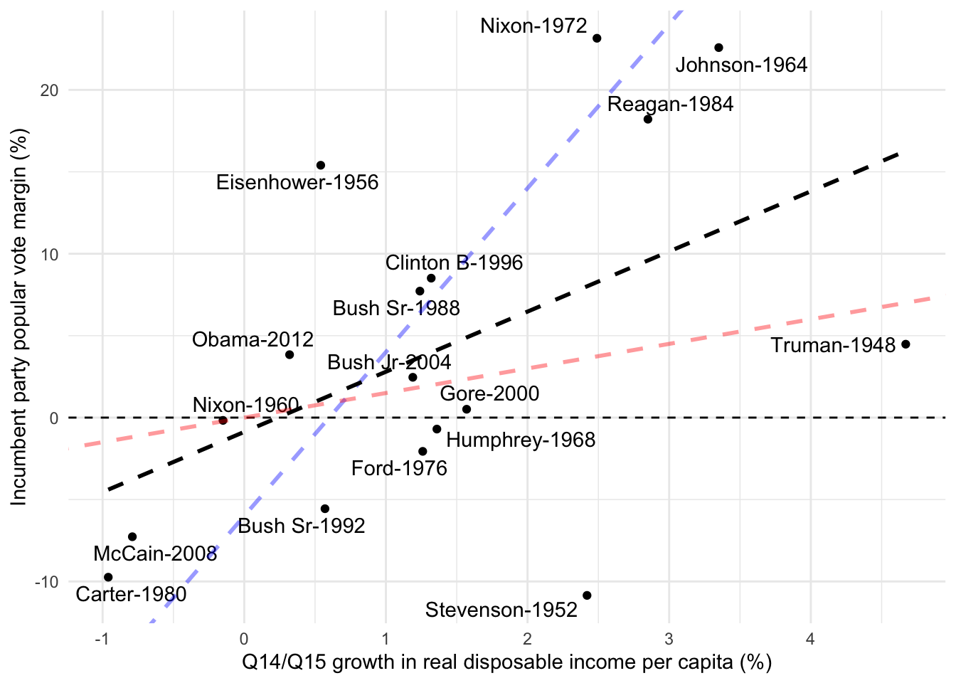
The goal of linear regression is to find the best-fitting straight line that represents the relationship between two variables based on the given data points. The “best fit” line is determined by minimizing the distance between the line and the actual data points. This distance is measured using residuals, which are the vertical distances from each data point to the line. The line that results in the smallest total residuals provides the best approximation of the relationship between the variables. For example, if we examine the plot below, we can observe that the red and blue lines do not fit the data points well, whereas the black line represents a better fit.
elec_plot +# One first "wrong" regression linegeom_abline(intercept =-6,slope =10,color ="blue",linetype ="dashed",size =1,alpha =0.4 ) +# A second "wrong" regression linegeom_abline(intercept =0,slope =1.5,color ="red",linetype ="dashed",size =1,alpha =0.4 ) +# The true regression linegeom_smooth(method ="lm",linetype ="dashed",color ="black",se =FALSE,size =1,alpha =0.4 )
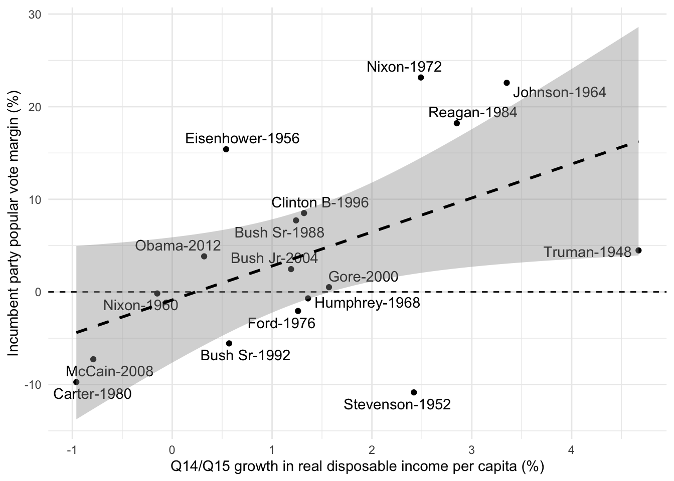
Linear regression not only provides us with the best-fitting line but also offers valuable information about the uncertainty associated with the estimated model parameters. This uncertainty is typically represented by confidence intervals around the regression line, which help us understand the range of possible values for the coefficients. Below, you can see this with the grey area around our regression line.
elec_plot +geom_smooth(method ="lm", linetype ="dashed", color ="black", se =TRUE, size =1, alpha =0.4)
14.2 Running a regression in R
Now we have a better idea of what a regression is, let’s run our first model. In R it is really easy to do ! You need to use the stats::lm() function. You need to insert a formula with on the left, the variable you want to explain and the right, the independent variables and in between, a ~. Before running the model, we have to make sure to know whether we have missing values or not in our data because the model will just drop them out and it is better to be aware of this.
model <-lm(elec$incm ~ elec$inc1415)model <-lm(incm ~ inc1415, data = elec)
To have a quick look at the results, you can use the summary() function. It provides you with the main results of the model.
summary(model)
Call:
lm(formula = incm ~ inc1415, data = elec)

Residuals:
    Min      1Q  Median      3Q     Max
-18.860  -5.343  -1.036   4.537  14.883

Coefficients:
            Estimate Std. Error t value Pr(>|t|)
(Intercept)  -0.8726     3.1754  -0.275   0.7872
inc1415       3.6707     1.6104   2.279   0.0377 *
---
Signif. codes:  0 '***' 0.001 '**' 0.01 '*' 0.05 '.' 0.1 ' ' 1

Residual standard error: 9.431 on 15 degrees of freedom
Multiple R-squared:  0.2573,    Adjusted R-squared:  0.2077
F-statistic: 5.196 on 1 and 15 DF,  p-value: 0.0377
But be aware that thare are in fact many more results that you can access. You can use the str() function to see all the results that you can access.
str(model)
List of 12
 $ coefficients : Named num [1:2] -0.873 3.671
  ..- attr(*, "names")= chr [1:2] "(Intercept)" "inc1415"
 $ residuals    : Named num [1:17] -11.79 -18.86 14.29 1.25 11.16 ...
  ..- attr(*, "names")= chr [1:17] "1" "2" "3" "4" ...
 $ effects      : Named num [1:17] -17.1 -21.5 12.7 -2.16 16.99 ...
  ..- attr(*, "names")= chr [1:17] "(Intercept)" "inc1415" "" "" ...
 $ rank         : int 2
 $ fitted.values: Named num [1:17] 16.27 8.01 1.11 -1.42 11.42 ...
  ..- attr(*, "names")= chr [1:17] "1" "2" "3" "4" ...
 $ assign       : int [1:2] 0 1
 $ qr           :List of 5
  ..$ qr   : num [1:17, 1:2] -4.123 0.243 0.243 0.243 0.243 ...
  .. ..- attr(*, "dimnames")=List of 2
  .. .. ..$ : chr [1:17] "1" "2" "3" "4" ...
  .. .. ..$ : chr [1:2] "(Intercept)" "inc1415"
  .. ..- attr(*, "assign")= int [1:2] 0 1
  ..$ qraux: num [1:2] 1.24 1.07
  ..$ pivot: int [1:2] 1 2
  ..$ tol  : num 1e-07
  ..$ rank : int 2
  ..- attr(*, "class")= chr "qr"
 $ df.residual  : int 15
 $ xlevels      : Named list()
 $ call         : language lm(formula = incm ~ inc1415, data = elec)
 $ terms        :Classes 'terms', 'formula'  language incm ~ inc1415
  .. ..- attr(*, "variables")= language list(incm, inc1415)
  .. ..- attr(*, "factors")= int [1:2, 1] 0 1
  .. .. ..- attr(*, "dimnames")=List of 2
  .. .. .. ..$ : chr [1:2] "incm" "inc1415"
  .. .. .. ..$ : chr "inc1415"
  .. ..- attr(*, "term.labels")= chr "inc1415"
  .. ..- attr(*, "order")= int 1
  .. ..- attr(*, "intercept")= int 1
  .. ..- attr(*, "response")= int 1
  .. ..- attr(*, ".Environment")=<environment: R_GlobalEnv>
  .. ..- attr(*, "predvars")= language list(incm, inc1415)
  .. ..- attr(*, "dataClasses")= Named chr [1:2] "numeric" "numeric"
  .. .. ..- attr(*, "names")= chr [1:2] "incm" "inc1415"
 $ model        :'data.frame':  17 obs. of  2 variables:
  ..$ incm   : num [1:17] 4.48 -10.85 15.4 -0.17 22.58 ...
  ..$ inc1415: num [1:17] 4.67 2.42 0.54 -0.15 3.35 1.36 2.49 1.26 -0.96 2.85 ...
  ..- attr(*, "terms")=Classes 'terms', 'formula'  language incm ~ inc1415
  .. .. ..- attr(*, "variables")= language list(incm, inc1415)
  .. .. ..- attr(*, "factors")= int [1:2, 1] 0 1
  .. .. .. ..- attr(*, "dimnames")=List of 2
  .. .. .. .. ..$ : chr [1:2] "incm" "inc1415"
  .. .. .. .. ..$ : chr "inc1415"
  .. .. ..- attr(*, "term.labels")= chr "inc1415"
  .. .. ..- attr(*, "order")= int 1
  .. .. ..- attr(*, "intercept")= int 1
  .. .. ..- attr(*, "response")= int 1
  .. .. ..- attr(*, ".Environment")=<environment: R_GlobalEnv>
  .. .. ..- attr(*, "predvars")= language list(incm, inc1415)
  .. .. ..- attr(*, "dataClasses")= Named chr [1:2] "numeric" "numeric"
  .. .. .. ..- attr(*, "names")= chr [1:2] "incm" "inc1415"
 - attr(*, "class")= chr "lm"
14.3 Extract and interpret the results
Once we have run the model, we first to extract and interpret the results. In R, you have different ways to look at and to manipulate the results of a regression model. Let’s look at them step by step.
14.3.1 Coefficients
First, you have the coefficients of the model that we have estimated. You can access directly the coefficient using the coef() function. An alternative way to see the results comes from the broom package (that you need to install and to load) that has super handy functions to get the results of the regression model in tidy format. The tidy() function allows you to extract the coefficient of the models and to get their confidence intervals and p values.
Our estimate for the intercept - 0.873. This means that if the Q14/Q15 growth in real disposable income per capita is 0, the incumbent party popular vote margin is -0.873. This means that on average, the incumbent party is losing the election when there is no economic growth.
Our estimate for for our first coefficient is 3.67. This is the slope of the regression line. That means that for each percentage point increase in growth in real disposable income per capita, the incumbent party popular vote margin increases by 3.67 percentage points.
statistic is the t.test. It is computed by dividing the coefficient by its standard error (3.67/1.61 = 2.28). The t.test is a measure of how many standard errors the coefficient is away from 0. If the t.test is >= 1.96, the coefficient will by statistically significant at the 5% level.
p.value :2 * (1 - pt(abs(2.28), 15)), df being the degree of freddom which our number of observations - our number of coefficients (17-2)
Looking at the p-value, we see that the p-value of our main esimate is inferior to 0.05, showing that it is stastically significant for this level of confidence.
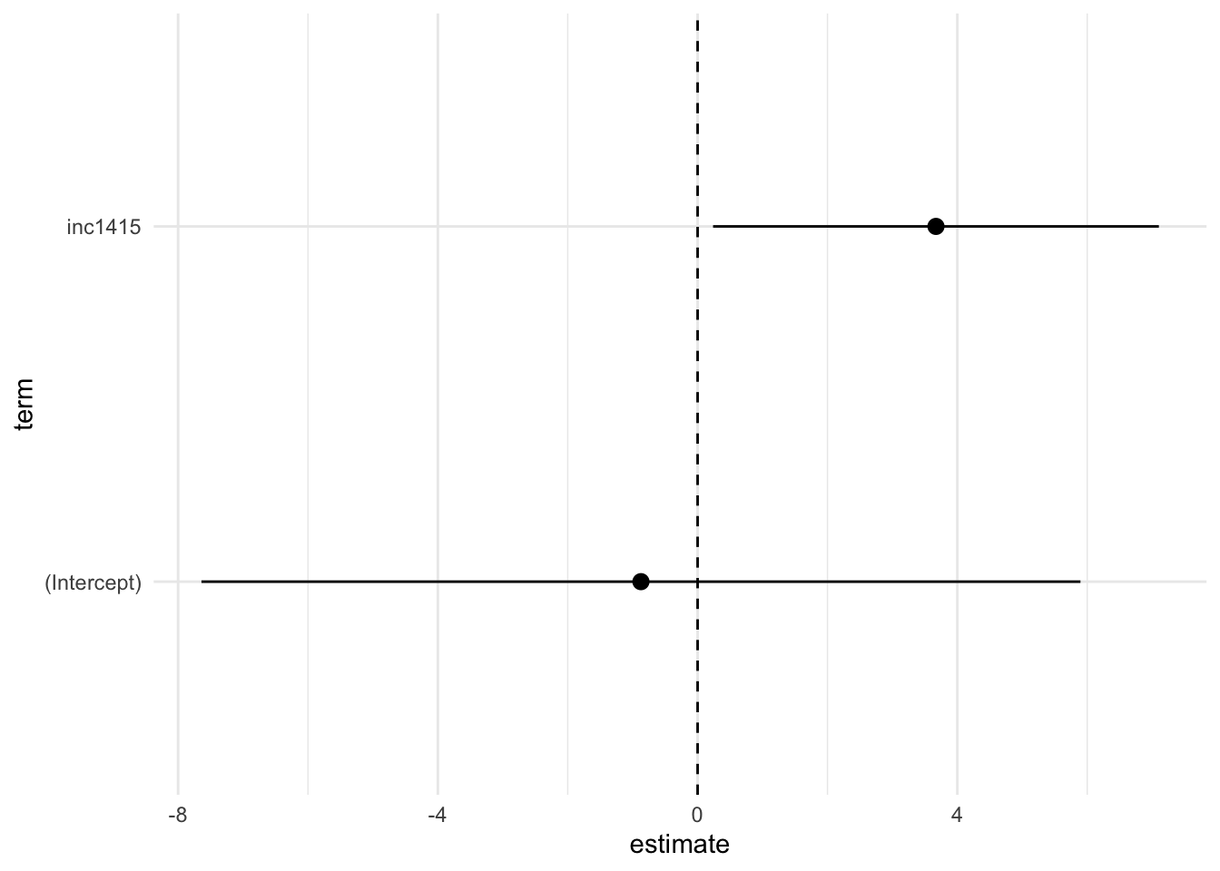
You can also use the output of tidy() to create coefficient plots. This is especially useful when you have many coefficients, and you want to quickly see which ones are significant or not. If the confidence interval bar crosses the dashed 0 line, it indicates that our coefficient will not be statistically significant. Remember that the sizes of coefficients are not directly comparable because they are not calculated on the same scale. The magnitude of each coefficient depends on the units of the corresponding independent variable. Therefore, comparing coefficients without considering their scales could lead to misleading interpretations. If you are lazy, you can use like coeffpot, dotwhisker, ggstat to create these plots. However, I personally favor creating them manually because it offers much more flexibility.
tidied |>ggplot(aes(x = term, y = estimate)) +# Create dot for our estimates with a bar for confidence intervalsgeom_pointrange(aes(ymin = conf.low, ymax = conf.high)) +# Create a dashed line at 0geom_hline(yintercept =0, linetype ="dashed") +coord_flip() +# invert y/x axestheme_minimal()
14.3.2 Model fit
When we run a regression, we also care about how good is our model to explain the variation of our outcome variable. The \(R^{2}\) is the amount of variation of our dependent variable that our model is able to explain. It goes from 0 to 1. If the \(R^{2}\) = 1, our model entirely explains Y (that will never happens). In social sciences we are happy with \(R^{2}\) of 0.2…
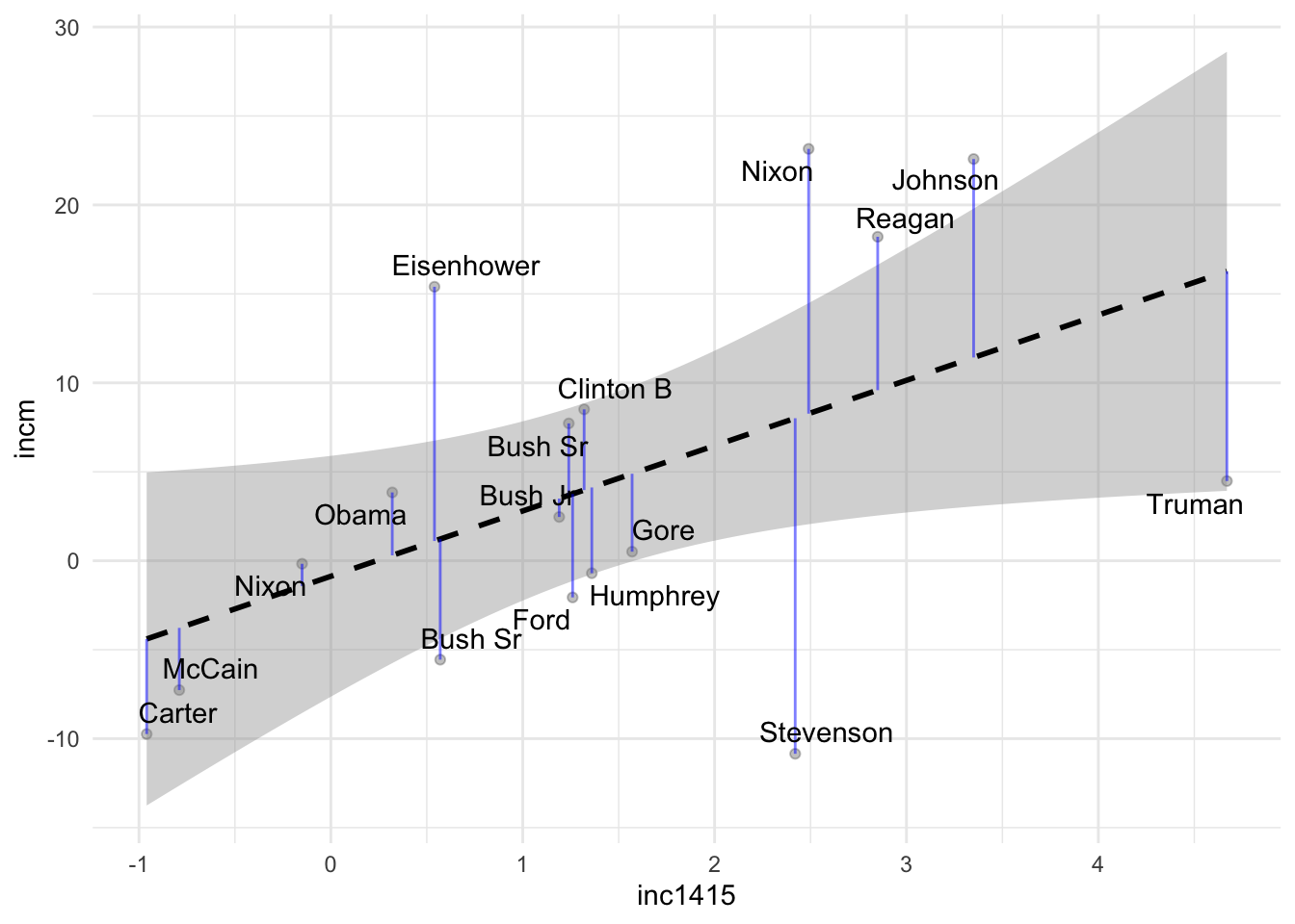
One last useful function from the broom package is augment(). This will give you the predictions of our model (our fitted values) and our residuals (the errors). This is useful to calculate different diagnostics that we will see in a further session.
The blue segments on the plot are the so-called residuals. These are the vertical distance between the ‘true’ value of our data to their fitted values on the regression line. The model is fitted by trying to minimize the sum of all of this distances.With this visualization, we can alo say something about how our model is doing to predict certain points. For instance, our model is doing a bad job at predicting the margins of victory of Einseihowever.
14.3.3 A note on categorical variables
We have seen that we can use continuous variables in our regression. But we can also use categorical variables. For instance, we can use the party_previous variable to understand the effect of being from one party or another on the margin of incumbent. Categorical variables have to be interepreted differently than continuous variables. The coefficient of a categorical variable is the difference between the mean of the outcome variable for the group of interest and the mean of the outcome variable for the reference group. Here, the reference group is Democrat. The coefficient of the party variable is the difference between the mean of the outcome variable for Republican and the mean of the outcome variable for Democrat. Here, our coefficient is 3.436 meaning that being from the Republican Party increases the margin of incumbent by 3.436 percentage points compared to being from the Democrat Party. However, our results are not statistically significant. Consequently, we cannot conclude that being from the Republican Party increases the margin of incumbent.
So far, we have tested the effect of two variables in two different models. However, we can also test the effect of two variables in a multiple linear regression model that allows us to control for the effect of other variables.
Call:
lm(formula = incm ~ inc1415 + party_previous, data = elec)

Residuals:
     Min       1Q   Median       3Q      Max
-16.0103  -5.3036  -0.9338   7.6383  13.4524

Coefficients:
                         Estimate Std. Error t value Pr(>|t|)
(Intercept)                -5.163      4.289  -1.204   0.2486
inc1415                     4.266      1.611   2.648   0.0191 *
party_previousRepublican    6.567      4.585   1.432   0.1740
---
Signif. codes:  0 '***' 0.001 '**' 0.01 '*' 0.05 '.' 0.1 ' ' 1

Residual standard error: 9.117 on 14 degrees of freedom
Multiple R-squared:  0.3522,    Adjusted R-squared:  0.2596
F-statistic: 3.805 on 2 and 14 DF,  p-value: 0.04788
We can also compare the fit our two models with glance() using the map_df function from the purrr package that is useful to apply a same function to different element of a list and return a tibble.
We can see that while our first model with the disposable income is doing a good job at explaining the variation of our outcome variable, our second model with the party variable is really bad. This is because the party variable is not a good predictor of the margin of incumbent. This is why we have a low \(R^{2}\).
Lastly, we can also look at our results in a regression table with the stargazer package.